STATS 220Data wrangling🛠1 / 64

Let's talk about code readability again!

looooooooooooooooong!

show_up_to_work(have_breakfast(glam_up(dress(shower(wake_up("I"))))))

infinite nesting......

show_up_to_work(
  have_breakfast(
    glam_up(
      dress(
        shower(
          wake_up("I")
        )
      )
    )
  )
)

2 / 64

data trans is beyond subsetting
reshape, summarise by groups
depends on Qs, the object of interest varies (from individual to aggregated level)
wrangle ur data to answer ur Qs
many funs involved
eg from we are rladies: morning routine
from wake up to go to work, interm steps

Does this one look better?

morning1 <- wake_up("I")
morning2 <- shower(morning1)
morning3 <- dress(morning2)
morning4 <- glam_up(morning3)
morning5 <- have_breakfast(morning4)
morning6 <- show_up_to_work(morning5)

many intermediate steps
not meaningful variable names

3 / 64

drain off naming ideas

Does this one look better?

morning1 <- wake_up("I")
morning2 <- shower(morning1)
morning3 <- dress(morning2)
morning4 <- glam_up(morning3)
morning5 <- have_breakfast(morning4)
morning6 <- show_up_to_work(morning5)

many intermediate steps
not meaningful variable names

How about this one?

morning_routine <- "I" %>% 
  wake_up() %>% 
  shower() %>% 
  dress() %>% 
  glam_up() %>% 
  have_breakfast() %>% 
  show_up_to_work()

%>% for expressing a linear sequence of multiple operations

3 / 64

drain off naming ideas

The code block: from a to z
ops are important to get your there
results from these inter ops will not be used.

RStudio shortcut: Ctrl/Cmd + Shift + M

4 / 64

r community, obsessed w 2 things
- pipe
- hex sticker
pipe originates from unix

Time use in OECD: 🛌 🏄‍♀️ 💇 👩‍🏫

library(readxl)
library(tidyverse)
time_use_raw <- read_xlsx("data/time-use-oecd.xlsx")
time_use_raw

#> # A tibble: 461 x 3
#>   Country   Category  `Time (minutes)`
#>   <chr>     <chr>                <dbl>
#> 1 Australia Paid work             211.
#> 2 Austria   Paid work             280.
#> 3 Belgium   Paid work             194.
#> 4 Canada    Paid work             269.
#> 5 Denmark   Paid work             200.
#> 6 Estonia   Paid work             231.
#> # … with 455 more rows

5 / 64

how individuals spend their time in OECD countries

Pipe the input into the first argument in the function

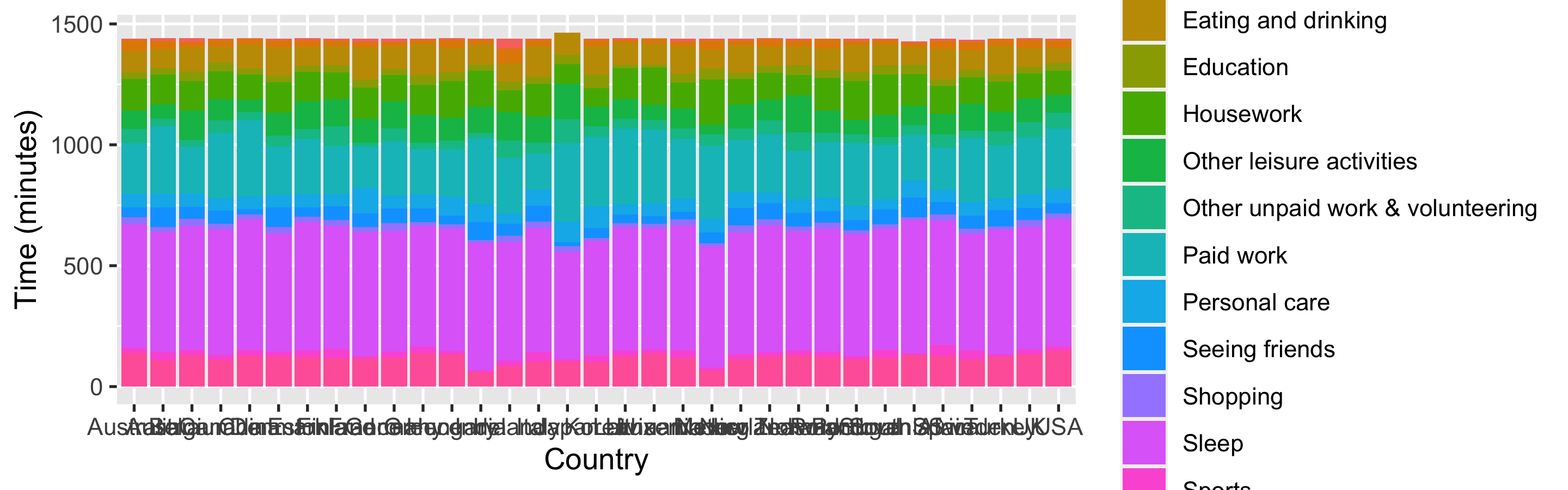
ggplot(time_use_raw) +
  geom_col(aes(
    Country, `Time (minutes)`, 
    fill = Category))

time_use_raw %>%
  ggplot() +
  geom_col(aes(
    Country, `Time (minutes)`, 
    fill = Category))

6 / 64

nvm, an awful plot
seems that there's one country with more time to spend
special characters: space and (), need backtick

Expressing yourself in

Hadley Wickham: Expressing yourself in R

7 / 64

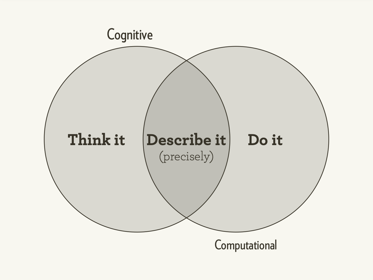
as ds, figure out what's your questions/what you want to do
translate your thoughts into code
let developers take care of computational side
the best or worst part of programming to precisely instruct computer to do what you want.
2017, hadley gave a talk

{dplyr} is a grammar of data manipulation, providing a consistent set of verbs that help you solve the most common data manipulation challenges:

mutate() adds new variables that are functions of existing variables
select() picks variables based on their names.
filter() picks cases based on their values.
summarise() reduces multiple values down to a single summary.
arrange() changes the ordering of the rows.

These all combine naturally with group_by() which allows you to perform any operation “by group”.

8 / 64

rowwise: filter obs and arrange obs
colwise
group-wise
succinct and expressive

One table verbs 🔨9 / 64

Rename columns

time_use <- time_use_raw %>% 
  rename( # new_name = old_name
    country = Country,
    category = Category, 
    minutes = `Time (minutes)`)
time_use

#> # A tibble: 461 x 3
#>   country   category  minutes
#>   <chr>     <chr>       <dbl>
#> 1 Australia Paid work    211.
#> 2 Austria   Paid work    280.
#> 3 Belgium   Paid work    194.
#> 4 Canada    Paid work    269.
#> 5 Denmark   Paid work    200.
#> 6 Estonia   Paid work    231.
#> # … with 455 more rows

10 / 64

although auto-comp is neat
deal w colnames many times: lower case, no space

Distinct rowstime_use %>% 
  distinct(category)

#> # A tibble: 14 x 1
#>    category                        
#>    <chr>                           
#>  1 Paid work                       
#>  2 Education                       
#>  3 Care for household members      
#>  4 Housework                       
#>  5 Shopping                        
#>  6 Other unpaid work & volunteering
#>  7 Sleep                           
#>  8 Eating and drinking             
#>  9 Personal care                   
#> 10 Sports                          
#> 11 Attending events                
#> 12 Seeing friends                  
#> 13 TV and Radio                    
#> 14 Other leisure activities
time_use %>% 
  distinct(country, category)

#> # A tibble: 461 x 2
#>   country   category 
#>   <chr>     <chr>    
#> 1 Australia Paid work
#> 2 Austria   Paid work
#> 3 Belgium   Paid work
#> 4 Canada    Paid work
#> 5 Denmark   Paid work
#> 6 Estonia   Paid work
#> # … with 455 more rows
11 / 64

massive data
check dups

Verbs

- rowwise

slice(): subsets rows using their positions

time_use %>% 
  slice((n() - 4):n())

#> # A tibble: 5 x 3
#>   country      category                 minutes
#>   <chr>        <chr>                      <dbl>
#> 1 UK           Other leisure activities    98.4
#> 2 USA          Other leisure activities    73.5
#> 3 China        Other leisure activities    53.0
#> 4 India        Other leisure activities   109. 
#> 5 South Africa Other leisure activities    81.8

n() is a context dependent function: the current group size

12 / 64

Verbs
- group by
group_by(): group by one or more variables

time_use %>% 
  group_by(country)

#> # A tibble: 461 x 3
#> # Groups:   country [33]
#>   country   category  minutes
#>   <chr>     <chr>       <dbl>
#> 1 Australia Paid work    211.
#> 2 Austria   Paid work    280.
#> 3 Belgium   Paid work    194.
#> 4 Canada    Paid work    269.
#> 5 Denmark   Paid work    200.
#> 6 Estonia   Paid work    231.
#> # … with 455 more rows
13 / 64

Verbs
- groupwise
group_by(): use in conjunction with other verbs

time_use %>% 
  group_by(country) %>% 
  slice((n() - 4):n())

#> # A tibble: 165 x 3
#> # Groups:   country [33]
#>   country   category                 minutes
#>   <chr>     <chr>                      <dbl>
#> 1 Australia Sports                     19.0 
#> 2 Australia Attending events            6.00
#> 3 Australia Seeing friends             40.0 
#> 4 Australia TV and Radio              140.  
#> 5 Australia Other leisure activities   76.1 
#> 6 Austria   Sports                     32.1 
#> # … with 159 more rows
14 / 64

Verbs
- groupwise
slice() shortcuts: slice_head() & slice_tail()

time_use %>% 
  group_by(country) %>% 
  slice_tail(n = 5)

#> # A tibble: 165 x 3
#> # Groups:   country [33]
#>   country   category                 minutes
#>   <chr>     <chr>                      <dbl>
#> 1 Australia Sports                     19.0 
#> 2 Australia Attending events            6.00
#> 3 Australia Seeing friends             40.0 
#> 4 Australia TV and Radio              140.  
#> 5 Australia Other leisure activities   76.1 
#> 6 Austria   Sports                     32.1 
#> # … with 159 more rows
15 / 64

Verbs
- group by
- ungroup
ungroup(): removes grouping

time_use %>% 
  group_by(country) %>% 
  slice_tail(n = 5) %>% 
  ungroup()

#> # A tibble: 165 x 3
#>   country   category                 minutes
#>   <chr>     <chr>                      <dbl>
#> 1 Australia Sports                     19.0 
#> 2 Australia Attending events            6.00
#> 3 Australia Seeing friends             40.0 
#> 4 Australia TV and Radio              140.  
#> 5 Australia Other leisure activities   76.1 
#> 6 Austria   Sports                     32.1 
#> # … with 159 more rows
16 / 64

Verbs
- rowwise
🌱slice_sample() randomly selects rows

set.seed(220) # an arbitrary number
time_use %>% 
  slice_sample(n = 10)

#> # A tibble: 10 x 3
#>    country     category                         minutes
#>    <chr>       <chr>                              <dbl>
#>  1 Norway      Housework                           82.9
#>  2 Austria     Education                           26.9
#>  3 Spain       Other leisure activities            84.7
#>  4 Estonia     Paid work                          231. 
#>  5 Canada      Education                           36.0
#>  6 Turkey      Education                           29.0
#>  7 Netherlands Housework                          105. 
#>  8 Australia   Sleep                              512. 
#>  9 Australia   Other unpaid work & volunteering    57.5
#> 10 Germany     Housework                          109.
17 / 64

random sampling
bootstrapping

Verbs

- rowwise

arrange(): arrange rows by columns

time_use %>% 
  arrange(minutes)

#> # A tibble: 461 x 3
#>   country   category                   minutes
#>   <chr>     <chr>                        <dbl>
#> 1 Japan     Care for household members    0   
#> 2 Lithuania Attending events              1.35
#> 3 China     Attending events              2.00
#> 4 Turkey    Attending events              2.58
#> 5 Poland    Attending events              2.81
#> 6 Korea     Attending events              4.45
#> # … with 455 more rows

arrange() in ascending order by default

18 / 64

Verbs

- rowwise

arrange(): arrange rows by columns

time_use %>% 
  arrange(desc(minutes)) # -minutes

#> # A tibble: 461 x 3
#>   country      category minutes
#>   <chr>        <chr>      <dbl>
#> 1 South Africa Sleep       553.
#> 2 China        Sleep       542.
#> 3 Estonia      Sleep       530.
#> 4 India        Sleep       528.
#> 5 USA          Sleep       528.
#> 6 New Zealand  Sleep       526 
#> # … with 455 more rows

use desc() in descending order

19 / 64

Verbs
- rowwise
arrange(): arrange rows by columns

time_use %>% 
  arrange(country, desc(minutes))

#> # A tibble: 461 x 3
#>   country   category                 minutes
#>   <chr>     <chr>                      <dbl>
#> 1 Australia Sleep                      512. 
#> 2 Australia Paid work                  211. 
#> 3 Australia TV and Radio               140. 
#> 4 Australia Housework                  132. 
#> 5 Australia Eating and drinking         89.1
#> 6 Australia Other leisure activities    76.1
#> # … with 455 more rows
20 / 64

Verbs

- rowwise

filter(): subsets rows using columns

time_use %>% 
  filter(minutes == max(minutes))

#> # A tibble: 1 x 3
#>   country      category minutes
#>   <chr>        <chr>      <dbl>
#> 1 South Africa Sleep       553.

filter() observations that satisfy your conditions

21 / 64

Verbs
- rowwise
filter(): subsets rows using columns

time_use %>% 
  group_by(country) %>% 
  filter(minutes == max(minutes))

#> # A tibble: 33 x 3
#> # Groups:   country [33]
#>   country   category minutes
#>   <chr>     <chr>      <dbl>
#> 1 Australia Sleep       512.
#> 2 Austria   Sleep       498.
#> 3 Belgium   Sleep       513.
#> 4 Canada    Sleep       520 
#> 5 Denmark   Sleep       489.
#> 6 Estonia   Sleep       530.
#> # … with 27 more rows
22 / 64

Verbs
- rowwise
filter(): subsets rows using columns

anz <- c("Australia", "New Zealand")
time_use %>% 
  filter(country %in% anz)

#> # A tibble: 28 x 3
#>   country     category                   minutes
#>   <chr>       <chr>                        <dbl>
#> 1 Australia   Paid work                    211. 
#> 2 New Zealand Paid work                    241. 
#> 3 Australia   Education                     27.0
#> 4 New Zealand Education                     29  
#> 5 Australia   Care for household members    44.5
#> 6 New Zealand Care for household members    30  
#> # … with 22 more rows
23 / 64

Verbs
- rowwise
filter(): subsets rows using columns

time_use %>% 
  filter(!(country %in% anz)) # ! logical negation (NOT)

#> # A tibble: 433 x 3
#>   country category  minutes
#>   <chr>   <chr>       <dbl>
#> 1 Austria Paid work    280.
#> 2 Belgium Paid work    194.
#> 3 Canada  Paid work    269.
#> 4 Denmark Paid work    200.
#> 5 Estonia Paid work    231.
#> 6 Finland Paid work    200.
#> # … with 427 more rows
24 / 64

Verbs
- rowwise
filter(): subsets rows using columns

time_use %>% 
  filter(country %in% anz, minutes > 30)
## time_use %>% 
##   filter(country %in% anz & minutes > 30)

#> # A tibble: 19 x 3
#>    country     category                         minutes
#>    <chr>       <chr>                              <dbl>
#>  1 Australia   Paid work                          211. 
#>  2 New Zealand Paid work                          241. 
#>  3 Australia   Care for household members          44.5
#>  4 Australia   Housework                          132. 
#>  5 New Zealand Housework                          110. 
#>  6 Australia   Other unpaid work & volunteering    57.5
#>  7 New Zealand Other unpaid work & volunteering    59  
#>  8 Australia   Sleep                              512. 
#>  9 New Zealand Sleep                              526  
#> 10 Australia   Eating and drinking                 89.1
#> 11 New Zealand Eating and drinking                 80  
#> 12 Australia   Personal care                       56.0
#> 13 New Zealand Personal care                       42  
#> 14 Australia   Seeing friends                      40.0
#> 15 New Zealand Seeing friends                      69  
#> 16 Australia   TV and Radio                       140. 
#> 17 New Zealand TV and Radio                       124  
#> 18 Australia   Other leisure activities            76.1
#> 19 New Zealand Other leisure activities            85
25 / 64

Verbs

- rowwise

filter(): subsets rows using columns

26 / 64

Verbs

- rowwise

filter(): subsets rows using columns

time_use %>% 
  filter(country %in% anz | minutes > 30)

#> # A tibble: 337 x 3
#>   country   category  minutes
#>   <chr>     <chr>       <dbl>
#> 1 Australia Paid work    211.
#> 2 Austria   Paid work    280.
#> 3 Belgium   Paid work    194.
#> 4 Canada    Paid work    269.
#> 5 Denmark   Paid work    200.
#> 6 Estonia   Paid work    231.
#> # … with 331 more rows

|: either ... or ...

27 / 64

Logical operatorsx <- c(TRUE, FALSE, TRUE, FALSE)
y <- c(FALSE, TRUE, TRUE, FALSE)

element-wise comparisons:

x & y

#> [1] FALSE FALSE  TRUE FALSE
x | y

#> [1]  TRUE  TRUE  TRUE FALSE
first-element only comparisons:

x && y

#> [1] FALSE
x || y

#> [1] TRUE
28 / 64

Verbs

- rowwise

filter(): subsets rows using columns

time_use_anz <- time_use %>% 
  filter(country %in% anz)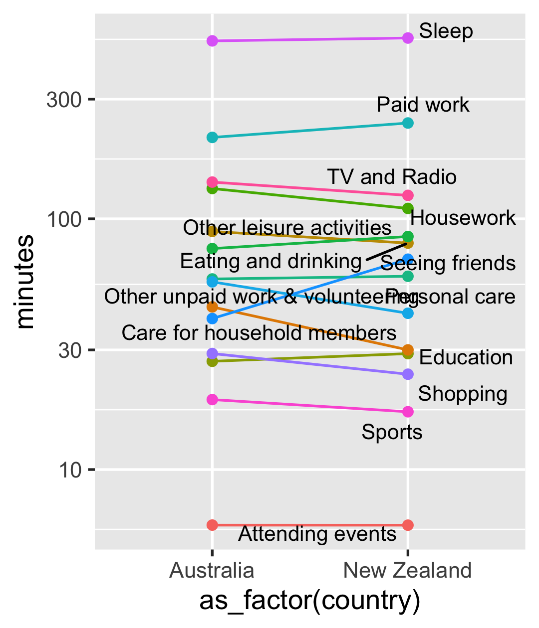

29 / 64

from now, started in looking at the anz data

Verbs
- rowwise
- colwise
select(): subsets columns using their names and types

time_use_anz %>% 
  select(country, category)
## time_use_anz %>% 
##   select(-minutes) # !minutes
## time_use_anz %>% 
##   select(country:category)

#> # A tibble: 28 x 2
#>   country     category                  
#>   <chr>       <chr>                     
#> 1 Australia   Paid work                 
#> 2 New Zealand Paid work                 
#> 3 Australia   Education                 
#> 4 New Zealand Education                 
#> 5 Australia   Care for household members
#> 6 New Zealand Care for household members
#> # … with 22 more rows
30 / 64

Verbs

- rowwise

- colwise

Selection helpers

starts_with(): starts with a prefix.
ends_with(): ends with a suffix.
contains(): contains a literal string.
more helpers

time_use_anz %>% 
  select(starts_with("c"))

#> # A tibble: 28 x 2
#>   country     category                  
#>   <chr>       <chr>                     
#> 1 Australia   Paid work                 
#> 2 New Zealand Paid work                 
#> 3 Australia   Education                 
#> 4 New Zealand Education                 
#> 5 Australia   Care for household members
#> 6 New Zealand Care for household members
#> # … with 22 more rows

31 / 64

Verbs
- rowwise
- colwise
mutate(): creates, modifies, and deletes columns

time_use_anz2 <- time_use_anz %>%
  mutate(
    # new_column = f(existing_column)
    hours = minutes / 60,
    iso = case_when(
      country == "Australia" ~ "AU", 
      TRUE ~ "NZ"))
time_use_anz2

#> # A tibble: 28 x 5
#>   country     category                   minutes hours iso  
#>   <chr>       <chr>                        <dbl> <dbl> <chr>
#> 1 Australia   Paid work                    211.  3.52  AU   
#> 2 New Zealand Paid work                    241.  4.02  NZ   
#> 3 Australia   Education                     27.0 0.450 AU   
#> 4 New Zealand Education                     29   0.483 NZ   
#> 5 Australia   Care for household members    44.5 0.742 AU   
#> 6 New Zealand Care for household members    30   0.5   NZ   
#> # … with 22 more rows
32 / 64

Verbs

- rowwise

- colwise

mutate(): creates, modifies, and deletes columns

33 / 64

`case_when()`: when it's the case, do something

z <- 1:10
case_when(
  # LHS ~ RHS
  # logical cond ~ replacement val
  z < 5 ~ "less than 5",
  z > 5 ~ "greater than 5",
  TRUE ~ "equal to 5"
)

#>  [1] "less than 5"    "less than 5"   
#>  [3] "less than 5"    "less than 5"   
#>  [5] "equal to 5"     "greater than 5"
#>  [7] "greater than 5" "greater than 5"
#>  [9] "greater than 5" "greater than 5"

34 / 64

Verbs
- rowwise
- colwise
summarise(): summarises to one row

time_use_anz2 %>% 
  summarise( # summarize()
    min = min(hours), 
    max = max(hours),
    avg = mean(hours))

#> # A tibble: 1 x 3
#>     min   max   avg
#>   <dbl> <dbl> <dbl>
#> 1   0.1  8.77  1.72
35 / 64

Verbs
- rowwise
- colwise
summarise(): summarises each group to fewer rows

time_use_anz2 %>% 
  group_by(category) %>% 
  summarise(
    min = min(hours), 
    max = max(hours),
    avg = mean(hours))

#> # A tibble: 14 x 4
#>    category                           min   max   avg
#>    <chr>                            <dbl> <dbl> <dbl>
#>  1 Attending events                 0.1   0.100 0.100
#>  2 Care for household members       0.5   0.742 0.621
#>  3 Eating and drinking              1.33  1.48  1.41 
#>  4 Education                        0.450 0.483 0.467
#>  5 Housework                        1.83  2.20  2.02 
#>  6 Other leisure activities         1.27  1.42  1.34 
#>  7 Other unpaid work & volunteering 0.959 0.983 0.971
#>  8 Paid work                        3.52  4.02  3.77 
#>  9 Personal care                    0.7   0.934 0.817
#> 10 Seeing friends                   0.667 1.15  0.908
#> 11 Shopping                         0.4   0.484 0.442
#> 12 Sleep                            8.54  8.77  8.65 
#> 13 Sports                           0.283 0.317 0.300
#> 14 TV and Radio                     2.07  2.33  2.20
36 / 64

Chain with %>%time_use_anz <- time_use %>% 
  filter(country %in% anz)

time_use_anz2 <- time_use_anz %>%
  mutate(
    # new_column = f(existing_column)
    hours = minutes / 60,
    iso = case_when(
      country == "Australia" ~ "AU", 
      TRUE ~ "NZ"))

time_use_anz2 %>% 
  group_by(category) %>% 
  summarise(
    min = min(hours), 
    max = max(hours),
    avg = mean(hours))

time_use %>% 
  filter(country %in% anz) %>% 
  mutate(hours = minutes / 60) %>% 
  group_by(category) %>% 
  summarise(
    min = min(hours), 
    max = max(hours), 
    avg = mean(hours))

37 / 64

When to %>%time_use %>% 
  filter(country %in% anz) %>% 
  mutate(hours = minutes / 60) %>% 
  group_by(category) %>% 
  summarise(
    min = min(hours), 
    max = max(hours), 
    avg = mean(hours))

Linear code dependency structure
< 10 steps
Inputs and outputs of the same type{dplyr} verbs, tibble in and out


38 / 64

The {tidyverse} is designed for data-centric tasks
a tibble in and a tibble out, that's why you can chain with %>%

Handy shortcuts

time_use_anz %>% 
  group_by(country) %>% 
  summarise(n = n())
## time_use_anz %>% 
##   count(country)
## time_use_anz %>% 
##   group_by(Country) %>% 
##   tally()

#> # A tibble: 2 x 2
#>   country         n
#>   <chr>       <int>
#> 1 Australia      14
#> 2 New Zealand    14

39 / 64

Hello again, SQL!

library(RSQLite)
con <- dbConnect(SQLite(), dbname = "data/pisa/pisa-student.db")
pisa_db <- tbl(con, "pisa")
pisa_db

#> # Source:   table<pisa> [?? x 22]
#> # Database: sqlite 3.34.1
#> #   [/Users/wany568/Teaching/stats220/lectures/data/pisa/pisa-student.db]
#>    year country school_id student_id mother_educ father_educ
#>   <dbl> <chr>   <chr>     <chr>      <chr>       <chr>      
#> 1  2000 ALB     1001      1          <NA>        <NA>       
#> 2  2000 ALB     1001      3          <NA>        <NA>       
#> 3  2000 ALB     1001      6          <NA>        <NA>       
#> 4  2000 ALB     1001      8          <NA>        <NA>       
#> 5  2000 ALB     1001      11         <NA>        <NA>       
#> 6  2000 ALB     1001      12         <NA>        <NA>       
#> # … with more rows, and 16 more variables: gender <chr>,
#> #   computer <chr>, internet <chr>, math <dbl>, read <dbl>,
#> #   science <dbl>, stu_wgt <dbl>, desk <chr>, room <chr>,
#> #   dishwasher <chr>, television <chr>, computer_n <chr>,
#> #   car <chr>, book <chr>, wealth <dbl>, escs <dbl>

40 / 64

Write {dplyr} code as usual to manipulate database

pisa_sql <- pisa_db %>% 
  filter(country %in% c("NZL", "AUS")) %>% 
  group_by(country) %>% 
  summarise(avg_math = mean(math, na.rm = TRUE)) %>% 
  arrange(desc(avg_math))
pisa_sql

#> # Source:     lazy query [?? x 2]
#> # Database:   sqlite 3.34.1
#> #   [/Users/wany568/Teaching/stats220/lectures/data/pisa/pisa-student.db]
#> # Ordered by: desc(avg_math)
#>   country avg_math
#>   <chr>      <dbl>
#> 1 NZL         511.
#> 2 AUS         502.

41 / 64

Speak in SQL from R

Show SQL queries

pisa_sql %>% show_query()

#> <SQL>
#> SELECT `country`, AVG(`math`) AS `avg_math`
#> FROM `pisa`
#> WHERE (`country` IN ('NZL', 'AUS'))
#> GROUP BY `country`
#> ORDER BY `avg_math` DESC

Retrieve results to R

pisa_sql %>% collect()

#> # A tibble: 2 x 2
#>   country avg_math
#>   <chr>      <dbl>
#> 1 NZL         511.
#> 2 AUS         502.

42 / 64

SQL is a beautiful and expressive language
dplyr is heavily inspired by SQL, but easier to use
as ds, you describe the data you want, and de write SQL to extract the data

Relational dataMultiple tables of data are called relational data because of the relations.43 / 64

Keys 🔑

A key is a variable (or set of variables) that uniquely identifies an observation.

A primary key uniquely identifies an observation in its own table.
A foreign key uniquely identifies an observation in another table.

time_use

#> # A tibble: 461 x 3
#>   country   category  minutes
#>   <chr>     <chr>       <dbl>
#> 1 Australia Paid work    211.
#> 2 Austria   Paid work    280.
#> 3 Belgium   Paid work    194.
#> 4 Canada    Paid work    269.
#> 5 Denmark   Paid work    200.
#> 6 Estonia   Paid work    231.
#> # … with 455 more rows

(country_code <- read_csv("data/countrycode.csv"))

#> # A tibble: 100 x 2
#>   country country_name
#>   <chr>   <chr>       
#> 1 AZE     Azerbaijan  
#> 2 ARG     Argentina   
#> 3 AUS     Australia   
#> 4 AUT     Austria     
#> 5 BEL     Belgium     
#> 6 BRA     Brazil      
#> # … with 94 more rows

44 / 64

Your turn

What's the key for the time_use data?

00:30

45 / 64

Two table verbs🤝46 / 64

A second data tableJoin country from country_code to time_use, by common values
Common values: country from time_use, but country_name from country_code
time_use %>% 
  filter(country %in% c("New Zealand", "USA")) %>% 
  distinct(country, .keep_all = TRUE)

#> # A tibble: 2 x 3
#>   country     category  minutes
#>   <chr>       <chr>       <dbl>
#> 1 New Zealand Paid work    241.
#> 2 USA         Paid work    251.
country_code %>% 
  filter(country_name %in% 
    c("New Zealand", "United States"))

#> # A tibble: 2 x 2
#>   country country_name 
#>   <chr>   <chr>        
#> 1 NZL     New Zealand  
#> 2 USA     United States
47 / 64

show 3 ways of printing

Joins

- mutating joins

Mutating joins: add new variables to one data frame from matching observations in another.

48 / 64

Joins

- mutating joins

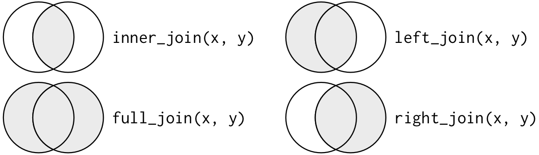
inner_join(): All rows from x where there are matching values in y, and all columns from x and y

image credit: Garrick Aden-Buie

49 / 64

Joins
- mutating joins
inner_join(): All rows from x where there are matching values in y, and all columns from x and y

time_use %>% 
  inner_join(country_code, by = c("country" = "country_name"))

#> # A tibble: 377 x 4
#>   country   category  minutes country.y
#>   <chr>     <chr>       <dbl> <chr>    
#> 1 Australia Paid work    211. AUS      
#> 2 Austria   Paid work    280. AUT      
#> 3 Belgium   Paid work    194. BEL      
#> 4 Canada    Paid work    269. CAN      
#> 5 Denmark   Paid work    200. DNK      
#> 6 Estonia   Paid work    231. EST      
#> # … with 371 more rows
50 / 64

live: leave by default
existing country column, dup name will be .y suffix

Joins

- mutating joins

left_join(): All rows from x, and all columns from x and y. Rows in x with no match in y will have NA values in the new columns.

image credit: Garrick Aden-Buie

51 / 64

Joins
- mutating joins
left_join(): All rows from x, and all columns from x and y. Rows in x with no match in y will have NA values in the new columns.

time_use %>% 
  left_join(country_code, by = c("country" = "country_name"))

#> # A tibble: 461 x 4
#>   country   category  minutes country.y
#>   <chr>     <chr>       <dbl> <chr>    
#> 1 Australia Paid work    211. AUS      
#> 2 Austria   Paid work    280. AUT      
#> 3 Belgium   Paid work    194. BEL      
#> 4 Canada    Paid work    269. CAN      
#> 5 Denmark   Paid work    200. DNK      
#> 6 Estonia   Paid work    231. EST      
#> # … with 455 more rows
52 / 64

Joins
- mutating joins
left_join(): All rows from x, and all columns from x and y. Rows in x with no match in y will have NA values in the new columns.

time_use %>% 
  left_join(country_code, by = c("country" = "country_name"))%>%
  filter(country %in% c("New Zealand", "USA")) %>% 
  group_by(country) %>% 
  slice_head()

#> # A tibble: 2 x 4
#> # Groups:   country [2]
#>   country     category  minutes country.y
#>   <chr>       <chr>       <dbl> <chr>    
#> 1 New Zealand Paid work    241. NZL      
#> 2 USA         Paid work    251. <NA>
53 / 64

Joins

- mutating joins

right_join(): All rows from y, and all columns from x and y. Rows in y with no match in x will have NA values in the new columns.

image credit: Garrick Aden-Buie

54 / 64

Joins
- mutating joins
right_join(): All rows from y, and all columns from x and y. Rows in y with no match in x will have NA values in the new columns.

time_use %>% 
  right_join(country_code, by = c("country" = "country_name"))

#> # A tibble: 450 x 4
#>   country   category  minutes country.y
#>   <chr>     <chr>       <dbl> <chr>    
#> 1 Australia Paid work    211. AUS      
#> 2 Austria   Paid work    280. AUT      
#> 3 Belgium   Paid work    194. BEL      
#> 4 Canada    Paid work    269. CAN      
#> 5 Denmark   Paid work    200. DNK      
#> 6 Estonia   Paid work    231. EST      
#> # … with 444 more rows
55 / 64

Joins

- mutating joins

full_join(): All rows and all columns from both x and y. Where there are not matching values, returns NA for the one missing.

image credit: Garrick Aden-Buie

56 / 64

Joins
- mutating joins
full_join(): All rows and all columns from both x and y. Where there are not matching values, returns NA for the one missing.

time_use %>% 
  full_join(country_code, by = c("country" = "country_name"))

#> # A tibble: 534 x 4
#>   country   category  minutes country.y
#>   <chr>     <chr>       <dbl> <chr>    
#> 1 Australia Paid work    211. AUS      
#> 2 Austria   Paid work    280. AUT      
#> 3 Belgium   Paid work    194. BEL      
#> 4 Canada    Paid work    269. CAN      
#> 5 Denmark   Paid work    200. DNK      
#> 6 Estonia   Paid work    231. EST      
#> # … with 528 more rows
57 / 64

Joins

- mutating joins

- filtering joins

Filtering joins: filter observations from one data frame based on whether or not they match an observation in the other table.

semi_join(): All rows from x where there are matching values in y, keeping just columns from x.

image credit: Garrick Aden-Buie

58 / 64

Joins
- mutating joins
- filtering joins
semi_join(): All rows from x where there are matching values in y, keeping just columns from x.

time_use %>% 
  semi_join(country_code, by = c("country" = "country_name"))

#> # A tibble: 377 x 3
#>   country   category  minutes
#>   <chr>     <chr>       <dbl>
#> 1 Australia Paid work    211.
#> 2 Austria   Paid work    280.
#> 3 Belgium   Paid work    194.
#> 4 Canada    Paid work    269.
#> 5 Denmark   Paid work    200.
#> 6 Estonia   Paid work    231.
#> # … with 371 more rows
59 / 64

Joins

- mutating joins

- filtering joins

anti_join(): All rows from x where there are not matching values in y, keeping just columns from x.

image credit: Garrick Aden-Buie

60 / 64

Joins
- mutating joins
- filtering joins
anti_join(): All rows from x where there are not matching values in y, keeping just columns from x.

time_use %>% 
  anti_join(country_code, by = c("country" = "country_name"))

#> # A tibble: 84 x 3
#>   country      category  minutes
#>   <chr>        <chr>       <dbl>
#> 1 Korea        Paid work    288.
#> 2 UK           Paid work    235.
#> 3 USA          Paid work    251.
#> 4 China        Paid work    315.
#> 5 India        Paid work    272.
#> 6 South Africa Paid work    189.
#> # … with 78 more rows
61 / 64

Useful functionsone table verbspull()
transmute()
relocate()

two table verbsbind_rows()
bind_cols()


set operationsunion()
union_all()
setdiff()
intersect()


62 / 64

Upcoming R-Ladies meetup

63 / 64

Reading

64 / 64

Help

Keyboard shortcuts

↑, ←, Pg Up, k

Go to previous slide

↓, →, Pg Dn, Space, j

Go to next slide

Home

Go to first slide

End

Go to last slide

Number + Return

Go to specific slide

b / m / f

Toggle blackout / mirrored / fullscreen mode

Clone slideshow

Toggle presenter mode

Restart the presentation timer

?, h

Toggle this help

STATS 220

Data wrangling🛠

Let's talk about code readability again!

Does this one look better?

Does this one look better?

How about this one?

Time use in OECD: 🛌 🏄‍♀️ 💇 👩‍🏫

Pipe the input into the first argument in the function

Expressing yourself in

One table verbs 🔨

Rename columns

Distinct rows

Verbs

- rowwise

Verbs

- group by

Verbs

- groupwise

Verbs

- groupwise

Verbs

- group by

- ungroup

Verbs

- rowwise

Verbs

- rowwise

Verbs

- rowwise

Verbs

- rowwise

Verbs

- rowwise

Verbs

- rowwise

Verbs

- rowwise

Verbs

- rowwise

Verbs

- rowwise

Verbs

- rowwise

Verbs

- rowwise

Logical operators

Verbs

- rowwise

Verbs

- rowwise

- colwise

Verbs

- rowwise

- colwise

Verbs

- rowwise

- colwise

Verbs

- rowwise

- colwise

case_when(): when it's the case, do something

Verbs

- rowwise

- colwise

Verbs

- rowwise

- colwise

Chain with %>%

When to %>%

Handy shortcuts

Hello again, SQL!

Write {dplyr} code as usual to manipulate database

Speak in SQL from R

Relational data

Multiple tables of data are called relational data because of the relations.

Keys 🔑

Your turn

Two table verbs🤝

A second data table

Joins

`case_when()`: when it's the case, do something

Chain with `%>%`

When to `%>%`