STATS 220

STATS 220🚀Factors & date-times📆1 / 31

2 / 31

forcats: my fav logo
lubridate: my fav pkg name

Atomic vectors

3 / 31

Coerce to factors from one type

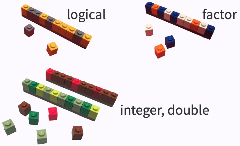
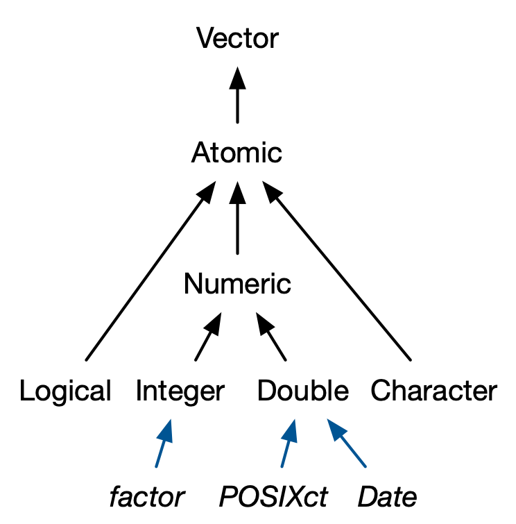
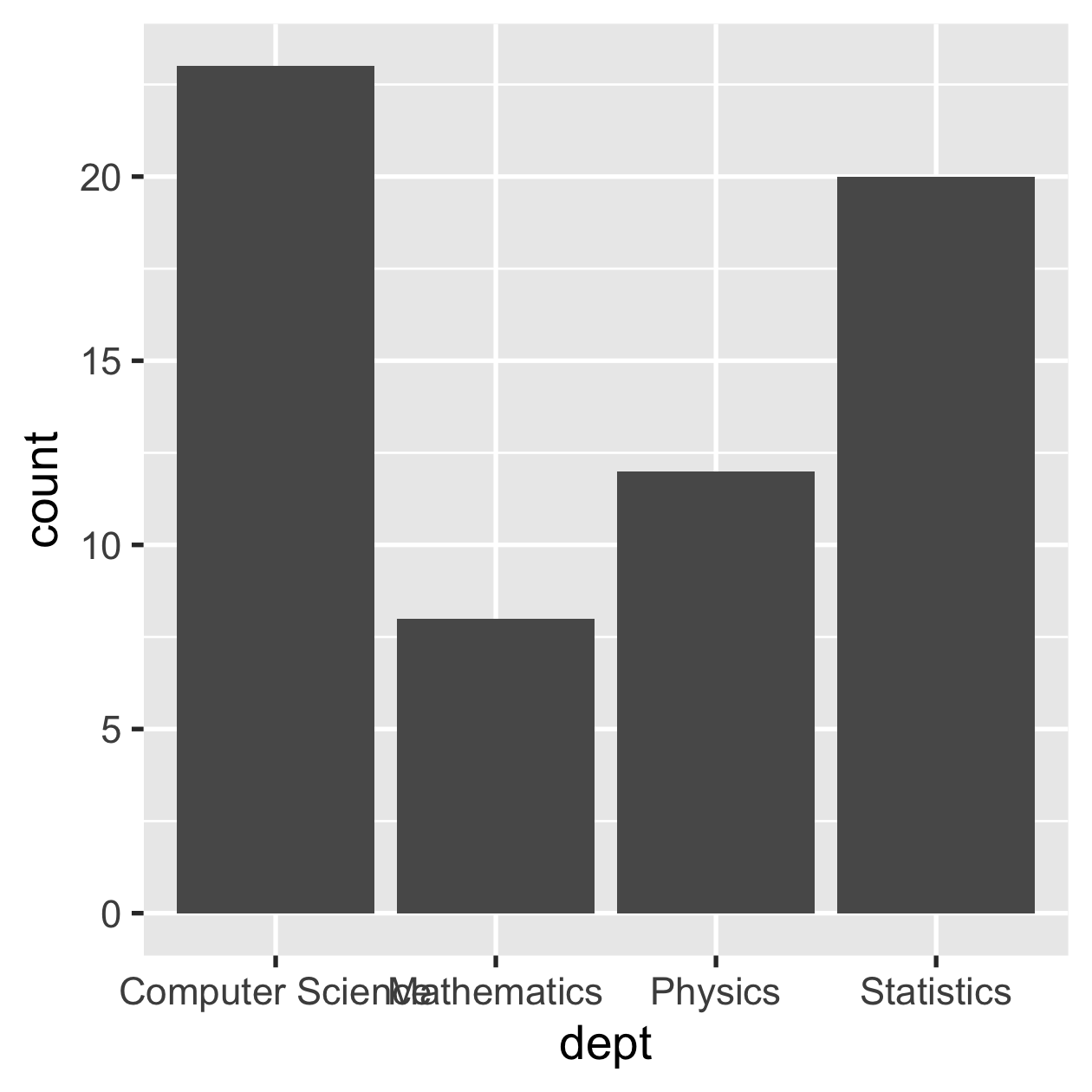
dept <- c("Physics", "Mathematics", "Statistics",
  "Computer Science")
dept

#> [1] "Physics"          "Mathematics"      "Statistics"      
#> [4] "Computer Science"

library(tidyverse) # library(forcats)
dept_fct <- as_factor(dept)
dept_fct

#> [1] Physics          Mathematics      Statistics      
#> [4] Computer Science
#> 4 Levels: Physics Mathematics ... Computer Science

4 / 31

diff displays
fct: w meta info

typeof(dept)

#> [1] "character"
class(dept)

#> [1] "character"
as.integer(dept)

#> [1] NA NA NA NA
sort(dept)

#> [1] "Computer Science"
#> [2] "Mathematics"     
#> [3] "Physics"         
#> [4] "Statistics"
typeof(dept_fct)

#> [1] "integer"
class(dept_fct)

#> [1] "factor"
as.integer(dept_fct)

#> [1] 1 2 3 4
sort(dept_fct)

#> [1] Physics          Mathematics     
#> [3] Statistics       Computer Science
#> 4 Levels: Physics ... Computer Science
5 / 31

FactorsFactors are used to represent a categorical variable in R.
There is a fixed and known set of possible values.
The fixed set of values is called the levels of the factor.
dept_fct

#> [1] Physics          Mathematics      Statistics       Computer Science
#> Levels: Physics Mathematics Statistics Computer Science
levels(dept_fct)

#> [1] "Physics"          "Mathematics"      "Statistics"       "Computer Science"
rep(dept_fct, 3)

#>  [1] Physics          Mathematics      Statistics       Computer Science
#>  [5] Physics          Mathematics      Statistics       Computer Science
#>  [9] Physics          Mathematics      Statistics       Computer Science
#> Levels: Physics Mathematics Statistics Computer Science
6 / 31

Create factors

change the base level for modelling
display characters in a non-alphabetical order

dist_dept <- unique(dept)
factor(dept, levels = dist_dept) # in first appearance order

#> [1] Physics          Mathematics      Statistics       Computer Science
#> Levels: Physics Mathematics Statistics Computer Science

factor(dept, levels = rev(dist_dept)) # in reverse order

#> [1] Physics          Mathematics      Statistics       Computer Science
#> Levels: Computer Science Statistics Mathematics Physics

7 / 31

data values not changing, only meta info levels changed

Reorder factor levels to easily perceive patterns

`sci_tbl`

8 / 31

in default order, takes time to process info

Reorder factor levels to easily perceive patterns

`movies`

9 / 31

`fct_reorder()` by sorting along another variable

sci_tbl %>% 
  mutate(dept = fct_reorder(dept, count)) %>%
  ggplot(aes(dept, count)) +
  geom_col()

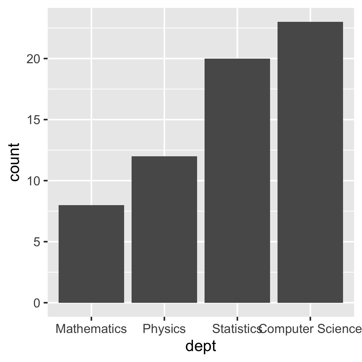
sci_tbl %>% 
  mutate(dept = fct_reorder(dept, -count)) %>%
  ggplot(aes(dept, count)) +
  geom_col()

10 / 31

`fct_reorder()` by sorting along another variable

fct_reorder(sci_tbl$dept, sci_tbl$count)

#> [1] Physics          Mathematics      Statistics       Computer Science
#> Levels: Mathematics Physics Statistics Computer Science

fct_reorder(sci_tbl$dept, -sci_tbl$count)

#> [1] Physics          Mathematics      Statistics       Computer Science
#> Levels: Computer Science Statistics Physics Mathematics

11 / 31

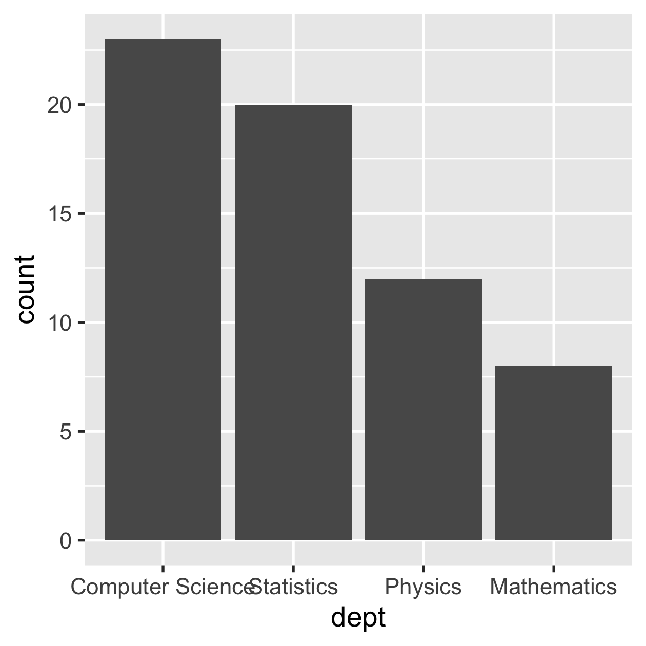
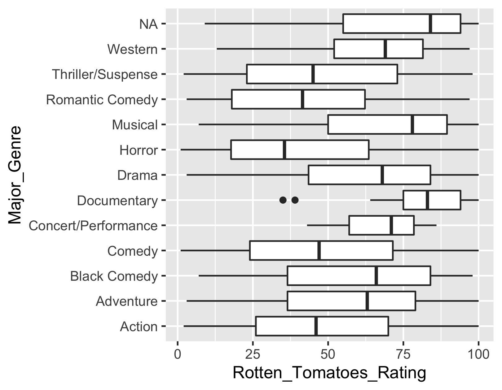
`fct_reorder()` by sorting along another variable with `fun()`

movies %>% 
  mutate(
    Major_Genre = fct_reorder(
      Major_Genre, 
      Rotten_Tomatoes_Rating,
      .fun = median, na.rm = TRUE)) %>%
  ggplot(aes(
    Rotten_Tomatoes_Rating, 
    Major_Genre)) +
  geom_boxplot()

12 / 31

`fct_infreq()` by counting obs with each level (largest first)

movies %>% 
  mutate(Major_Genre = fct_infreq(
    Major_Genre)) %>% 
  ggplot(aes(y = Major_Genre)) +
  geom_bar()

13 / 31

`fct_lump()` by lumping together factor levels into "other"

movies %>% 
  mutate(Major_Genre = fct_infreq(
    fct_lump(Major_Genre, n = 6))) %>%
  ggplot(aes(y = Major_Genre)) +
  geom_bar()

14 / 31

Convert numerics to factors: UoA grade scales

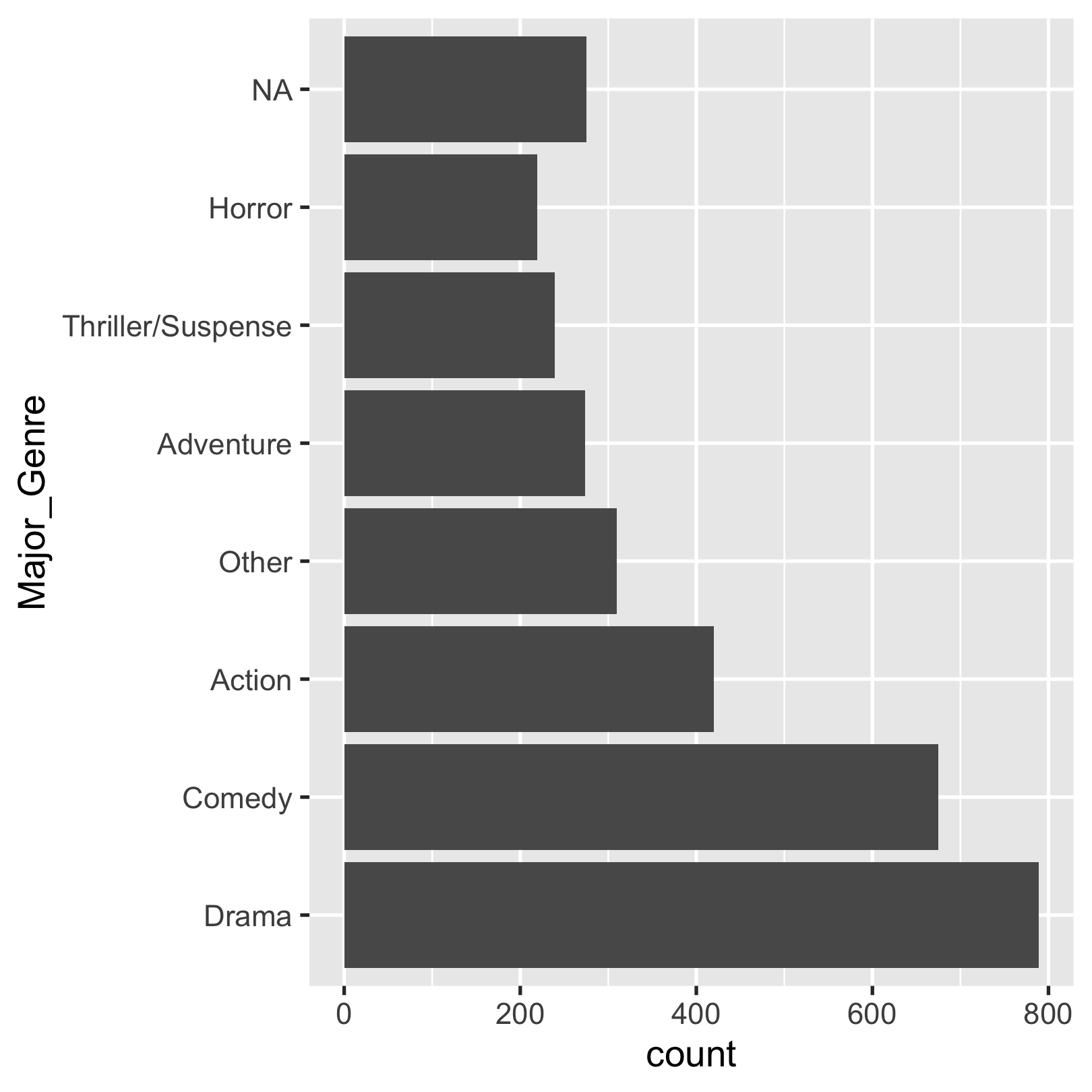
set.seed(220)
scores_sim <- round(
  rnorm(309, mean = 70, sd = 10),
  digits = 2)
scores_tbl <- tibble(score = scores_sim)
scores_tbl

#> # A tibble: 309 x 1
#>   score
#>   <dbl>
#> 1  58.2
#> 2  80.1
#> 3  51.4
#> 4  80.5
#> 5  63.8
#> 6  51.0
#> # … with 303 more rows

scores_tbl %>% 
  ggplot(aes(x = score)) +
  geom_histogram() +
  geom_vline(xintercept = 70, 
    colour = "red")

15 / 31

`cut()` numerics to factors

(rng <- c(0, seq(39, 89, by = 5), 100))

#>  [1]   0  39  44  49  54  59  64  69  74  79  84  89 100

scores_tbl %>% 
  mutate(range = cut(score, breaks = rng, include.lowest = TRUE))

#> # A tibble: 309 x 2
#>   score range  
#>   <dbl> <fct>  
#> 1  58.2 (54,59]
#> 2  80.1 (79,84]
#> 3  51.4 (49,54]
#> 4  80.5 (79,84]
#> 5  63.8 (59,64]
#> 6  51.0 (49,54]
#> # … with 303 more rows

16 / 31

underappreciated cut(), built-in function
include 0, but doesn't matter for this data

`fct_recode()` changes factor levels by hand

scores_schemes <- scores_tbl %>% 
  mutate(
    range = cut(score, breaks = rng, include.lowest = TRUE),
    grade = fct_recode(range, # new_lvl = old_lvl
      "D-" = "[0,39]", "D" = "(39,44]", "D+" = "(44,49]",
      "C-" = "(49,54]", "C" = "(54,59]", "C+" = "(59,64]",
      "B-" = "(64,69]", "B" = "(69,74]", "B+" = "(74,79]",
      "A-" = "(79,84]", "A" = "(84,89]", "A+" = "(89,100]"))
scores_schemes

#> # A tibble: 309 x 3
#>   score range   grade
#>   <dbl> <fct>   <fct>
#> 1  58.2 (54,59] C    
#> 2  80.1 (79,84] A-   
#> 3  51.4 (49,54] C-   
#> 4  80.5 (79,84] A-   
#> 5  63.8 (59,64] C+   
#> 6  51.0 (49,54] C-   
#> # … with 303 more rows

17 / 31

Here I show the fct_recode(), manual work
what's other way to do this quickly

scores_schemes %>% 
  ggplot(aes(x = range)) +
  geom_bar()

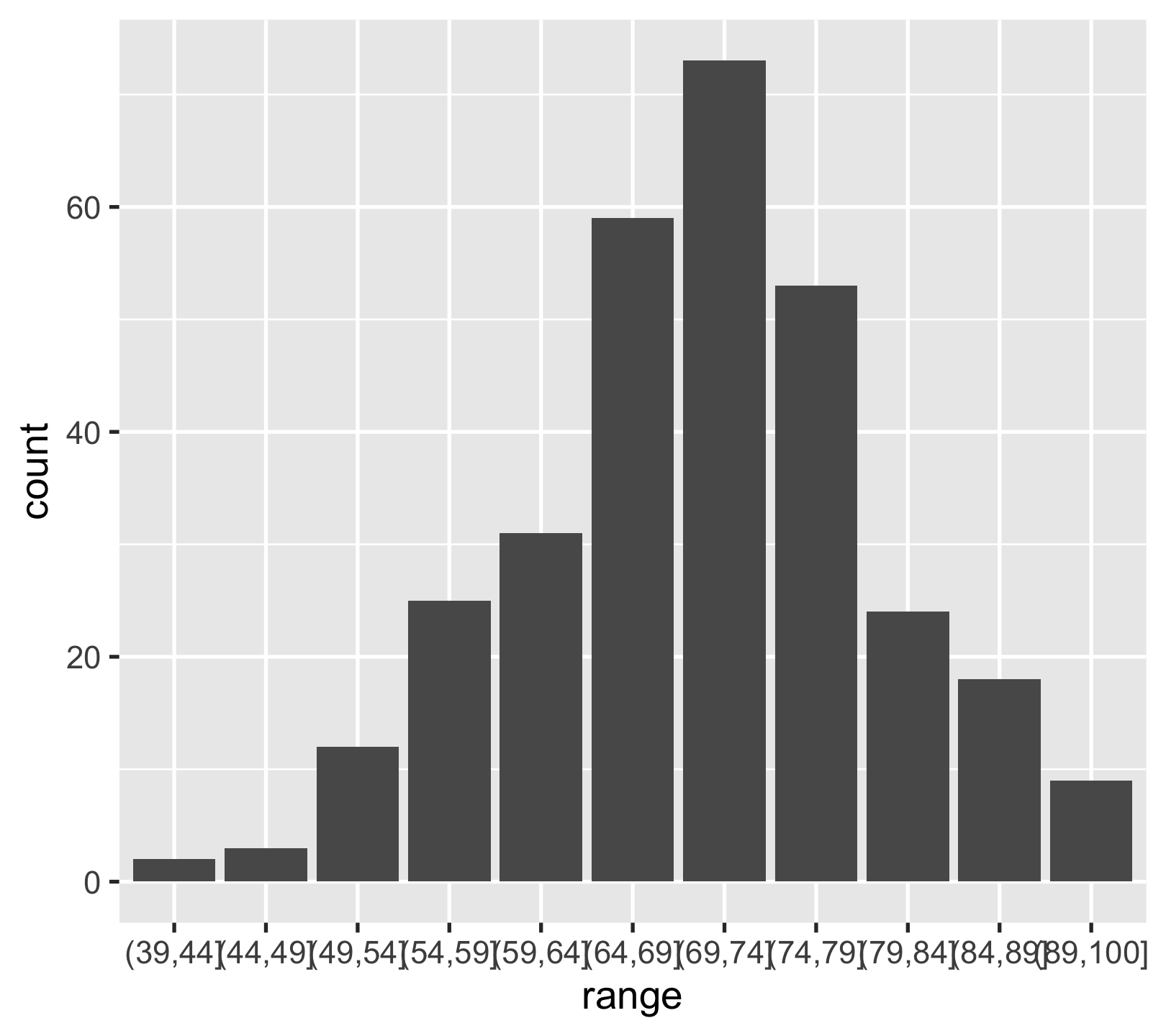
scores_schemes %>% 
  ggplot(aes(x = grade)) +
  geom_bar()

18 / 31

Your turn

What function can we use to replace fct_recode() for the scores_tbl data?

00:30

19 / 31

live demo: fct_rev()

⬇️ {lubridate} is NOT part of the core {tidyverse}, so load with

library(lubridate)

Relative and exact time units:

An instant is a specific moment in time, such as January 1st, 2012.
An interval is a period of time that occurs between two specific instants.
A duration records the time span in seconds, it will have an exact length since seconds always have the same length.
A period records a time span in units larger than seconds, such as years, months, weeks, days, hours, and minutes.

20 / 31

temporal data (recorded over time) is everywhere. Ur phone tracks your daily life.
instant: timestamp
leap seconds/years, time zones, DST
lab04, tz

📆Dates
(td <- today())

#> [1] "2021-03-31"
class(td)

#> [1] "Date"
typeof(td)

#> [1] "double"
as.integer(td) # 1970-01-01

#> [1] 18717
⌚Date-times
(current <- now())

#> [1] "2021-03-31 12:22:35 NZDT"
class(current)

#> [1] "POSIXct" "POSIXt"
typeof(current)

#> [1] "double"
as.integer(current) # 1970-01-01 00:00:00

#> [1] 1617146555
21 / 31

Create date-times

make_date(2021, c(3, 6), c(31, 4))

#> [1] "2021-03-31" "2021-06-04"

make_datetime(2021, c(3, 6), c(31, 4), c(16, 10))

#> [1] "2021-03-31 16:00:00 UTC" "2021-06-04 10:00:00 UTC"

make_datetime(2021, c(3, 6), c(31, 4), c(16, 10), tz = "Pacific/Auckland")

#> [1] "2021-03-31 16:00:00 NZDT" "2021-06-04 10:00:00 NZST"

22 / 31

Available time zones (~ 600‼️)

set.seed(220)
OlsonNames()[sample(1:length(OlsonNames()), 32)]

#>  [1] "Pacific/Midway"                 "Africa/Asmera"                 
#>  [3] "Africa/Lusaka"                  "ROK"                           
#>  [5] "America/Montreal"               "Europe/Dublin"                 
#>  [7] "Asia/Irkutsk"                   "Africa/Cairo"                  
#>  [9] "Asia/Dubai"                     "America/Yellowknife"           
#> [11] "Asia/Tbilisi"                   "America/Menominee"             
#> [13] "Atlantic/Azores"                "GMT-0"                         
#> [15] "America/Louisville"             "Europe/Astrakhan"              
#> [17] "Pacific/Fakaofo"                "America/Nome"                  
#> [19] "Etc/GMT+10"                     "Pacific/Efate"                 
#> [21] "GB-Eire"                        "Asia/Thimphu"                  
#> [23] "US/Eastern"                     "Europe/Busingen"               
#> [25] "Australia/NSW"                  "America/Hermosillo"            
#> [27] "MET"                            "Pacific/Enderbury"             
#> [29] "America/Argentina/Rio_Gallegos" "Asia/Ashgabat"                 
#> [31] "Africa/Dakar"                   "Canada/Atlantic"

23 / 31

Parse date-times

ymd(c("2021/03/31", "2021-June-04"))

#> [1] "2021-03-31" "2021-06-04"

ymd_h(c("2021-03-31 16", "2021-June-04 10"))

#> [1] "2021-03-31 16:00:00 UTC" "2021-06-04 10:00:00 UTC"

(dttm <- ymd_h(c("2021-03-31 16", "2021-June-04 10"), tz = "Pacific/Auckland"))

#> [1] "2021-03-31 16:00:00 NZDT" "2021-06-04 10:00:00 NZST"

ymd(), ymd_h(), ymd_hm(), ymd_hms()
dmy(), dmy_h(), dmy_hm(), dmy_hms()

mdy(), mdy_h(), mdy_hm(), mdy_hms()

24 / 31

Extract components of date-timesdate(dttm)

#> [1] "2021-03-31" "2021-06-04"
year(dttm)

#> [1] 2021 2021
yday(dttm)

#> [1]  90 155
week(dttm)

#> [1] 13 23
day(dttm) # mday(dttm)

#> [1] 31  4
hour(dttm)

#> [1] 16 10
minute(dttm)

#> [1] 0 0
second(dttm)

#> [1] 0 0
25 / 31

Extract months/weekdays of date-timesmonth

month(dttm)

#> [1] 3 6
month(dttm, label = TRUE)

#> [1] Mar Jun
#> 12 Levels: Jan < Feb < Mar < ... < Dec
weekday

wday(dttm, week_start = 1)

#> [1] 3 5
wday(dttm, label = TRUE)

#> [1] Wed Fri
#> 7 Levels: Sun < Mon < Tue < ... < Sat
wday(dttm, label = TRUE, week_start = 1)

#> [1] Wed Fri
#> 7 Levels: Mon < Tue < Wed < ... < Sun
26 / 31

Round, floor and ceiling date-times

floor_date(dttm, "3 hours")

#> [1] "2021-03-31 15:00:00 NZDT" "2021-06-04 09:00:00 NZST"

ceiling_date(dttm, "2 days")

#> [1] "2021-04-02 NZDT" "2021-06-05 NZST"

round_date(dttm, "1 month")

#> [1] "2021-04-01 NZDT" "2021-06-01 NZST"

27 / 31

Perform accurate math on date-timesdttm + 1

#> [1] "2021-03-31 16:00:01 NZDT"
#> [2] "2021-06-04 10:00:01 NZST"
dttm + minutes(2)

#> [1] "2021-03-31 16:02:00 NZDT"
#> [2] "2021-06-04 10:02:00 NZST"
dttm + hours(3)

#> [1] "2021-03-31 19:00:00 NZDT"
#> [2] "2021-06-04 13:00:00 NZST"
dttm + days(4)

#> [1] "2021-04-04 16:00:00 NZST"
#> [2] "2021-06-08 10:00:00 NZST"
dttm + weeks(5)

#> [1] "2021-05-05 16:00:00 NZST"
#> [2] "2021-07-09 10:00:00 NZST"
dttm + months(6)

#> [1] NA                        
#> [2] "2021-12-04 10:00:00 NZDT"
dttm + years(7)

#> [1] "2028-03-31 16:00:00 NZDT"
#> [2] "2028-06-04 10:00:00 NZST"
28 / 31

Format date-times (also coerce to characters)format(dttm)

#> [1] "2021-03-31 16:00:00" "2021-06-04 10:00:00"
format(dttm, "%Y/%b/%d")

#> [1] "2021/Mar/31" "2021/Jun/04"
format(dttm, "%y/%b/%d %H:%M:%S")

#> [1] "21/Mar/31 16:00:00" "21/Jun/04 10:00:00"
format(dttm, "on %d %B (%a)")

#> [1] "on 31 March (Wed)" "on 04 June (Fri)"
a/A: Abbreviated/full weekday name.
b/B: Abbreviated or full month name.
m: Month as decimal number (01-12 or 1-12).
d: Day of the month as decimal number (01-31 or 0-31)
w: Weekday as decimal number (0-6, Sunday is 0).
y/Y: Year without/with century.
more on ?parse_date_time()

29 / 31

📽`movies`

movies$Release_Date[c(38:39, 268)]

#> [1] "18-Oct-06"  "1963-01-01" NA

movies %>% 
  mutate(
    Release_Date = parse_date_time(
      Release_Date, c("%d-%b-%y", "%Y-%m-%d")),
    Year = year(Release_Date)
  ) %>% 
  filter(Year < 2012) %>% 
  ggplot(aes(Year, IMDB_Rating)) +
  geom_hex()

30 / 31

Reading

31 / 31

Help

Keyboard shortcuts

↑, ←, Pg Up, k

Go to previous slide

↓, →, Pg Dn, Space, j

Go to next slide

Home

Go to first slide

End

Go to last slide

Number + Return

Go to specific slide

b / m / f

Toggle blackout / mirrored / fullscreen mode

Clone slideshow

Toggle presenter mode

Restart the presentation timer

?, h

Toggle this help

STATS 220

🚀Factors & date-times📆

Atomic vectors

Coerce to factors from one type

Factors

Create factors

Reorder factor levels to easily perceive patterns

sci_tbl

Reorder factor levels to easily perceive patterns

movies

fct_reorder() by sorting along another variable

fct_reorder() by sorting along another variable

fct_reorder() by sorting along another variable with fun()

fct_infreq() by counting obs with each level (largest first)

fct_lump() by lumping together factor levels into "other"

Convert numerics to factors: UoA grade scales

cut() numerics to factors

fct_recode() changes factor levels by hand

Your turn

📆Dates

⌚Date-times

Create date-times

Available time zones (~ 600‼️)

Parse date-times

Extract components of date-times

Extract months/weekdays of date-times

Round, floor and ceiling date-times

Perform accurate math on date-times

Format date-times (also coerce to characters)

📽movies

Reading

Help

`sci_tbl`

`movies`

`fct_reorder()` by sorting along another variable

`fct_reorder()` by sorting along another variable

`fct_reorder()` by sorting along another variable with `fun()`

`fct_infreq()` by counting obs with each level (largest first)

`fct_lump()` by lumping together factor levels into "other"

`cut()` numerics to factors

`fct_recode()` changes factor levels by hand

📽`movies`