STATS 220

STATS 220Tidy data🧹1 / 36

2 / 36

image sources: Upsplash

2 / 36

each piece is a scalar, a vector, a tibble, a list
each piece is vector functions or table functions
bc they are standard and consistent blocks,
ensemble them to a simple mario, or complex nintendo
so far you worked with several datasets now,
hopefully you find a pattern is using these dplyr verbs in different ways to solve various problems.

What you think about data science 🤩

image credit: Hilary Parker

3 / 36

80% on modelling

What data science is in reality 😭

image credit: Hilary Parker

4 / 36

80% on cleaning
it's invaluable to know the data pipeline: how data collected and organised
covid19, different def for each country in the early stage

tidy data clean data

The movies data is tidy but not clean.

#> # A tibble: 5 x 16
#>   Release_Date US_DVD_Sales Title      US_Gross Worldwide_Gross Production_Budg…
#>   <chr>               <int> <chr>         <int>           <dbl>            <int>
#> 1 9-Mar-94               NA Four Wedd… 52700832       242895809          4500000
#> 2 18-Oct-06              NA 51 Birch …    84689           84689           350000
#> 3 1963-01-01             NA 55 Days a… 10000000        10000000         17000000
#> 4 <NA>                   NA Drei              0               0          7200000
#> 5 16-Jan-98              NA The Dress     16556           16556          2650000
#> # … with 10 more variables: MPAA_Rating <chr>, Running_Time_min <int>,
#> #   Distributor <chr>, Source <chr>, Major_Genre <chr>, Creative_Type <chr>,
#> #   Director <chr>, Rotten_Tomatoes_Rating <int>, IMDB_Rating <dbl>,
#> #   IMDB_Votes <int>

5 / 36

all data you've seen so far are tidy, but tidy doesn't mean clean.
how I would clean this data:
either google Drei release year, and corresponding GDP
or replace GDP with NA
Gross are suspicious

tidy data clean data

They are tidy and clean in their own way.

time_use

#> # A tibble: 28 x 3
#>   country    category            minutes
#>   <chr>      <chr>                 <dbl>
#> 1 New Zeala… Paid work             241  
#> 2 USA        Paid work             251. 
#> 3 New Zeala… Education              29  
#> 4 USA        Education              31.4
#> 5 New Zeala… Care for household…    30  
#> 6 USA        Care for household…    30.6
#> # … with 22 more rows

countrycode

#> # A tibble: 2 x 2
#>   country country_name 
#>   <chr>   <chr>        
#> 1 NZL     New Zealand  
#> 2 USA     United States

6 / 36

week 4, when we try to join them, we see how country names are encoded differently.
Data cleaning is laborious, and highly dependent on the data itself.
No golden standards or principles to guide how to clean data.
reason about the cleaning steps (intuition, common sense, business context)
principles to get tidy data.

Tidy data describes a standard way of storing data in a consistent format.7 / 36

tidy data is about data format, instead of caring the data values.

Your turn

Tuberculosis data from WHO (data/tb.csv):

Is tb tidy data?
What are the data observations? What are the data variables?

tb

#> # A tibble: 5,769 x 22
#>   iso2   year  m_04 m_514 m_014 m_1524 m_2534 m_3544 m_4554 m_5564  m_65   m_u
#>   <chr> <dbl> <dbl> <dbl> <dbl>  <dbl>  <dbl>  <dbl>  <dbl>  <dbl> <dbl> <dbl>
#> 1 AD     1989    NA    NA    NA     NA     NA     NA     NA     NA    NA    NA
#> 2 AD     1990    NA    NA    NA     NA     NA     NA     NA     NA    NA    NA
#> 3 AD     1991    NA    NA    NA     NA     NA     NA     NA     NA    NA    NA
#> 4 AD     1992    NA    NA    NA     NA     NA     NA     NA     NA    NA    NA
#> 5 AD     1993    NA    NA    NA     NA     NA     NA     NA     NA    NA    NA
#> 6 AD     1994    NA    NA    NA     NA     NA     NA     NA     NA    NA    NA
#> # … with 5,763 more rows, and 10 more variables: f_04 <dbl>, f_514 <dbl>,
#> #   f_014 <dbl>, f_1524 <dbl>, f_2534 <dbl>, f_3544 <dbl>, f_4554 <dbl>,
#> #   f_5564 <dbl>, f_65 <dbl>, f_u <dbl>

01:00

8 / 36

Can you easily plot a dataset like this using ggplot2? by sex and age
come back later

one data, many representations

image credit: Garrick Aden-Buie

9 / 36

which rep does tb resemble?
which rep is easier to work with? depends on the question, wide -> suitable for summary table

10 / 36

In database, this is schema.
Tidy data principles are a rephrase of third norm in a database schema design. https://en.wikipedia.org/wiki/Third_normal_form, to data scientists.
tidy data is for human consumption.
Tabular data is column-oriented format

11 / 36

Making friends with tidy data

one set of consistent tools for different datasets
easier for automation and iteration

reference: Illustrations from the Openscapes blog Tidy Data for reproducibility, efficiency, and collaboration by Julia Lowndes and Allison Horst

12 / 36

To work with messy data, every time you need to switch to different gears
learn new tools that just works for that specific dataset
It's much more pleasant to work with tidy data, help you to build a good taste of data analysis
spent less flighting with different tools, focus more on data analysis bc one set of consistent tools
the {tidyverse} philosophy to work with the tidy data structures
build automatic workflow for analysis, feed different data sets.

Get data into tidy format

type	`function()`	`function()`
pivoting	`pivot_longer()`	`pivot_wider()`
splitting/combining	`seperate()`	`unite()`
nesting/unnesting	`nest()`	`unnest()`
missing	`complete()`	`fill()`

13 / 36

missing verbs not exactly a pair

Messy

#> # A tibble: 5,769 x 22
#>   iso2   year  m_04 m_514 m_014
#>   <chr> <dbl> <dbl> <dbl> <dbl>
#> 1 AD     1989    NA    NA    NA
#> 2 AD     1990    NA    NA    NA
#> 3 AD     1991    NA    NA    NA
#> 4 AD     1992    NA    NA    NA
#> 5 AD     1993    NA    NA    NA
#> 6 AD     1994    NA    NA    NA
#> # … with 5,763 more rows, and 17
#> #   more variables: m_1524 <dbl>,
#> #   m_2534 <dbl>, m_3544 <dbl>,
#> #   m_4554 <dbl>, m_5564 <dbl>,
#> #   m_65 <dbl>, m_u <dbl>,
#> #   f_04 <dbl>, f_514 <dbl>,
#> #   f_014 <dbl>, f_1524 <dbl>,
#> #   f_2534 <dbl>, f_3544 <dbl>,
#> #   f_4554 <dbl>, f_5564 <dbl>,
#> #   f_65 <dbl>, f_u <dbl>
Tidy

#> # A tibble: 115,380 x 5
#>   iso2   year sex   age   cases
#>   <chr> <dbl> <chr> <chr> <dbl>
#> 1 AD     1989 m     04        0
#> 2 AD     1989 m     514       0
#> 3 AD     1989 m     014       0
#> 4 AD     1989 m     1524      0
#> 5 AD     1989 m     2534      0
#> 6 AD     1989 m     3544      0
#> # … with 115,374 more rows
14 / 36

the tb data is messy data, rows and columns
obs and variables
working with tidy data, we know obs: the number of cases by sex and age groups over years at country level
messy in a way that column names should be values, stored in cells.
what steps needed to get to this tidy format.

- pivot

pivot_longer() a wider-format data

library(tidyverse) # library(tidyr)
tb %>% 
  pivot_longer(
    cols = m_04:f_u, # cols in the data for pivoting
    names_to = "sex_age", # new col contains old headers
    values_to = "cases") # new col contains old values

#> # A tibble: 115,380 x 4
#>   iso2   year sex_age cases
#>   <chr> <dbl> <chr>   <dbl>
#> 1 AD     1989 m_04       NA
#> 2 AD     1989 m_514      NA
#> 3 AD     1989 m_014      NA
#> 4 AD     1989 m_1524     NA
#> 5 AD     1989 m_2534     NA
#> 6 AD     1989 m_3544     NA
#> # … with 115,374 more rows

15 / 36

messy: store two variables into one column

- pivot

image credit: Garrick Aden-Buie & Mara Averick

16 / 36

- pivot

- split

seperate() a character column into multiple columns

tb %>% 
  pivot_longer(cols = m_04:f_u, 
    names_to = "sex_age", values_to = "cases") %>% 
  separate(sex_age, into = c("sex", "age"), sep = "_")

#> # A tibble: 115,380 x 5
#>   iso2   year sex   age   cases
#>   <chr> <dbl> <chr> <chr> <dbl>
#> 1 AD     1989 m     04       NA
#> 2 AD     1989 m     514      NA
#> 3 AD     1989 m     014      NA
#> 4 AD     1989 m     1524     NA
#> 5 AD     1989 m     2534     NA
#> 6 AD     1989 m     3544     NA
#> # … with 115,374 more rows

17 / 36

- pivot

- split

- fill

fill() in NA with previous ("down") or next ("up") value

tb_tidy <- tb %>% 
  pivot_longer(cols = m_04:f_u, 
    names_to = "sex_age", values_to = "cases") %>% 
  separate(sex_age, into = c("sex", "age"), sep = "_") %>% 
  group_by(iso2) %>% 
  fill(cases, .direction = "updown") %>%
  ungroup()

#> # A tibble: 115,380 x 5
#>   iso2   year sex   age   cases
#>   <chr> <dbl> <chr> <chr> <dbl>
#> 1 AD     1989 m     04        0
#> 2 AD     1989 m     514       0
#> 3 AD     1989 m     014       0
#> 4 AD     1989 m     1524      0
#> 5 AD     1989 m     2534      0
#> 6 AD     1989 m     3544      0
#> # … with 115,374 more rows

18 / 36

how to impute missing data is dependent on data context. For cross-sectional, average and build a regression model to predict
fill by direction
demo on direction

- pivot

- split

- fill

- nest

nest() multiple columns into a list-column

tb_tidy %>% 
  nest(data = -iso2)

#> # A tibble: 213 x 2
#>   iso2  data                  
#>   <chr> <list>                
#> 1 AD    <tibble[,4] [380 × 4]>
#> 2 AE    <tibble[,4] [520 × 4]>
#> 3 AF    <tibble[,4] [480 × 4]>
#> 4 AG    <tibble[,4] [540 × 4]>
#> 5 AI    <tibble[,4] [440 × 4]>
#> 6 AL    <tibble[,4] [540 × 4]>
#> # … with 207 more rows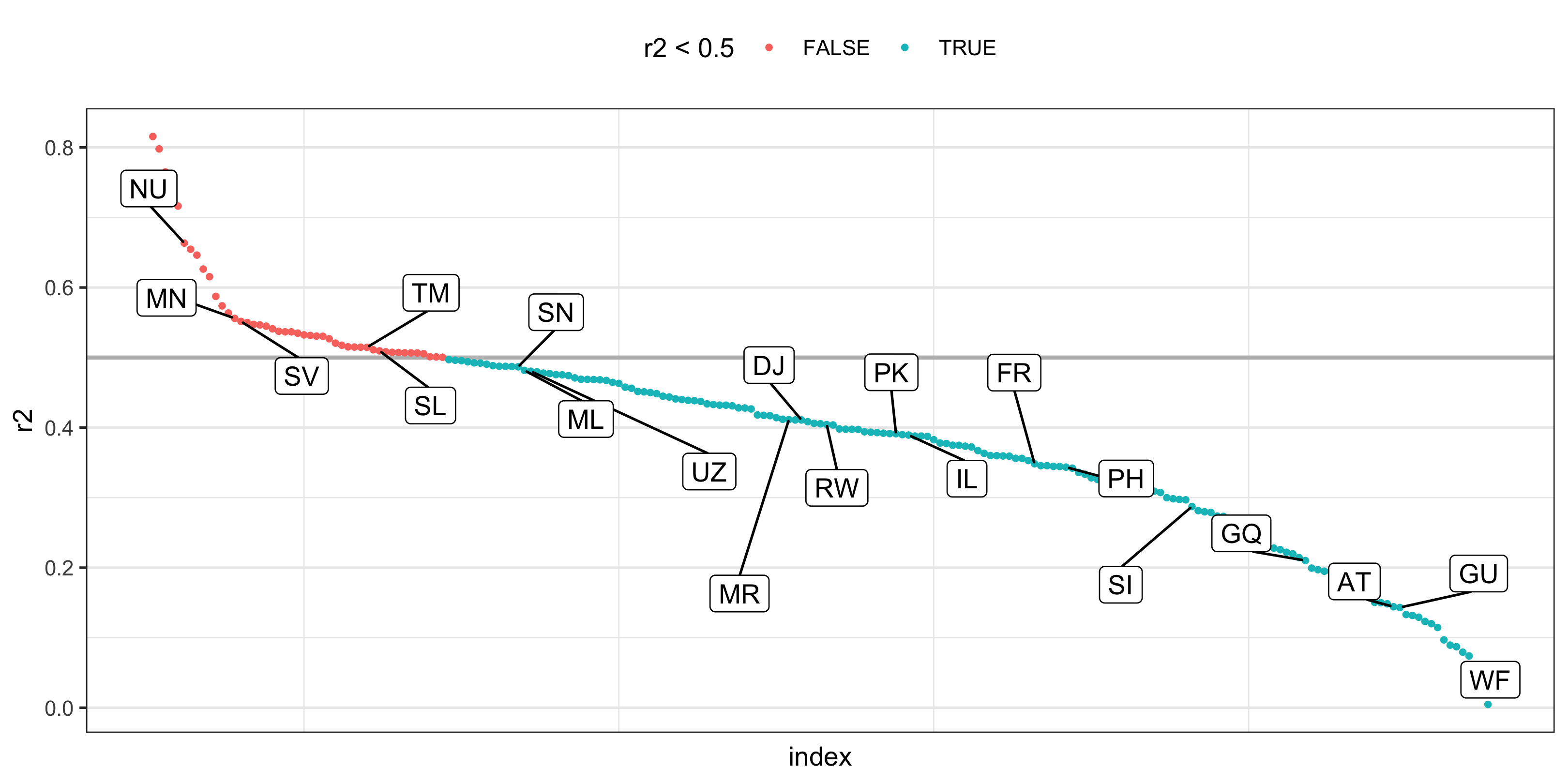

19 / 36

tibble is a list, recursive structure
we can put a list into a tibble
complex objs in tibble

Building many models*

tb_fit <- tb_tidy %>% 
  nest(data = -iso2) %>% 
  mutate( # map() for week 11
    model = map(data, ~ lm(cases ~ year + sex + age, data = .)),
    r2 = map_dbl(model, ~ broom::glance(.)$r.squared)
  )

#> # A tibble: 213 x 4
#>   iso2  data                   model     r2
#>   <chr> <list>                 <list> <dbl>
#> 1 AD    <tibble[,4] [380 × 4]> <lm>   0.165
#> 2 AE    <tibble[,4] [520 × 4]> <lm>   0.133
#> 3 AF    <tibble[,4] [480 × 4]> <lm>   0.487
#> 4 AG    <tibble[,4] [540 × 4]> <lm>   0.220
#> 5 AI    <tibble[,4] [440 × 4]> <lm>   0.515
#> 6 AL    <tibble[,4] [540 × 4]> <lm>   0.478
#> # … with 207 more rows

20 / 36

r2 for each country

set.seed(220)
tb_fit_pre <- tb_fit %>% 
  arrange(-r2) %>% 
  mutate(iso2 = fct_inorder(iso2), index = row_number())
hl_tb <- tb_fit_pre %>% 
  slice_sample(n = 20)
tb_fit_pre %>% 
  ggplot(aes(x = index, y = r2)) +
  geom_hline(yintercept = 0.5, size = 0.8, colour = "grey") +
  geom_point(aes(colour = r2 < 0.5), size = 0.8) +
  ggrepel::geom_label_repel(aes(label = iso2), data = hl_tb, box.padding = 1) +
  theme_bw() +
  theme(
    axis.text.x = element_blank(),
    axis.ticks.x = element_blank(),
    panel.grid.major.x = element_blank(),
    legend.position = "top"
  )

21 / 36

direct labeling instead of > 200 country labels underneath

Your turn

Auckland weather data from GHCND (data/ghcnd/ghcnd-akl.csv):

Is aklweather tidy data?
What are the data observations? What are the data variables?

aklweather

#> # A tibble: 2,974 x 3
#>   date       datatype value
#>   <date>     <chr>    <dbl>
#> 1 2019-01-01 PRCP         0
#> 2 2019-01-01 TAVG       206
#> 3 2019-01-01 TMAX       232
#> 4 2019-01-01 TMIN       188
#> 5 2019-01-02 PRCP         5
#> 6 2019-01-02 TAVG       207
#> # … with 2,968 more rows

01:00

22 / 36

The value column contains multiple types of measurements.

Messy

#> # A tibble: 2,974 x 3
#>   date       datatype value
#>   <date>     <chr>    <dbl>
#> 1 2019-01-01 PRCP         0
#> 2 2019-01-01 TAVG       206
#> 3 2019-01-01 TMAX       232
#> 4 2019-01-01 TMIN       188
#> 5 2019-01-02 PRCP         5
#> 6 2019-01-02 TAVG       207
#> # … with 2,968 more rows
aklweather <- read_csv2(
  "data/ghcnd/ghcnd-akl.csv",
  col_types = cols_only(
    date = "D", datatype = "c", 
    value = "d"))
aklweather
Tidy

#> # A tibble: 816 x 5
#>   date        PRCP  TAVG  TMAX  TMIN
#>   <date>     <dbl> <dbl> <dbl> <dbl>
#> 1 2019-01-01     0   206   232   188
#> 2 2019-01-02     5   207   230   183
#> 3 2019-01-03     0   211   241   184
#> 4 2019-01-04     0   192   229    NA
#> 5 2019-01-05     0   200   233   150
#> 6 2019-01-06     0   213   237   169
#> # … with 810 more rows
23 / 36

demo on read_csv2()
daily weather information in Auckland
temp values unbelievably large?

- calibrate

calibrate the measurements

aklweather %>%
  mutate(value = value / 10)

#> # A tibble: 2,974 x 3
#>   date       datatype value
#>   <date>     <chr>    <dbl>
#> 1 2019-01-01 PRCP       0  
#> 2 2019-01-01 TAVG      20.6
#> 3 2019-01-01 TMAX      23.2
#> 4 2019-01-01 TMIN      18.8
#> 5 2019-01-02 PRCP       0.5
#> 6 2019-01-02 TAVG      20.7
#> # … with 2,968 more rows

24 / 36

- calibrate

- pivot

pivot_wider() a longer-format data

aklweather %>%
  mutate(value = value / 10) %>% 
  pivot_wider(
    names_from = datatype, # new headers from old `datatype` val
    values_from = value)  # new col contains old `value`

#> # A tibble: 816 x 5
#>   date        PRCP  TAVG  TMAX  TMIN
#>   <date>     <dbl> <dbl> <dbl> <dbl>
#> 1 2019-01-01   0    20.6  23.2  18.8
#> 2 2019-01-02   0.5  20.7  23    18.3
#> 3 2019-01-03   0    21.1  24.1  18.4
#> 4 2019-01-04   0    19.2  22.9  NA  
#> 5 2019-01-05   0    20    23.3  15  
#> 6 2019-01-06   0    21.3  23.7  16.9
#> # … with 810 more rows

25 / 36

- calibrate

- pivot

26 / 36

- calibrate

- pivot

- rename

rename_with() renames columns using a function

aklweather_tidy <- aklweather %>%
  mutate(value = value / 10) %>% 
  pivot_wider(
    names_from = datatype,
    values_from = value) %>%
  rename_with(tolower)
aklweather_tidy

#> # A tibble: 816 x 5
#>   date        prcp  tavg  tmax  tmin
#>   <date>     <dbl> <dbl> <dbl> <dbl>
#> 1 2019-01-01   0    20.6  23.2  18.8
#> 2 2019-01-02   0.5  20.7  23    18.3
#> 3 2019-01-03   0    21.1  24.1  18.4
#> 4 2019-01-04   0    19.2  22.9  NA  
#> 5 2019-01-05   0    20    23.3  15  
#> 6 2019-01-06   0    21.3  23.7  16.9
#> # … with 810 more rows

27 / 36

tedious to type

- calibrate

- pivot

- rename

- complete

complete() data with missing combinations of data

library(lubridate)
aklweather_tidy %>% 
  complete(date = full_seq(
    ymd(c("2019-01-01", "2021-04-01")), 1))

#> # A tibble: 822 x 5
#>   date        prcp  tavg  tmax  tmin
#>   <date>     <dbl> <dbl> <dbl> <dbl>
#> 1 2019-01-01   0    20.6  23.2  18.8
#> 2 2019-01-02   0.5  20.7  23    18.3
#> 3 2019-01-03   0    21.1  24.1  18.4
#> 4 2019-01-04   0    19.2  22.9  NA  
#> 5 2019-01-05   0    20    23.3  15  
#> 6 2019-01-06   0    21.3  23.7  16.9
#> # … with 816 more rows

28 / 36

- calibrate

- pivot

- rename

- complete

implicit missing records before

aklweather_tidy %>% 
  complete(date = full_seq(
    ymd(c("2019-01-01", "2021-04-01")), 1)) %>% 
  anti_join(aklweather_tidy)

#> # A tibble: 6 x 5
#>   date        prcp  tavg  tmax  tmin
#>   <date>     <dbl> <dbl> <dbl> <dbl>
#> 1 2019-02-16    NA    NA    NA    NA
#> 2 2019-02-17    NA    NA    NA    NA
#> 3 2019-02-18    NA    NA    NA    NA
#> 4 2021-02-11    NA    NA    NA    NA
#> 5 2021-02-12    NA    NA    NA    NA
#> 6 2021-02-20    NA    NA    NA    NA

29 / 36

implicit bf, explicit after complete()

- calibrate

- pivot

- rename

- complete

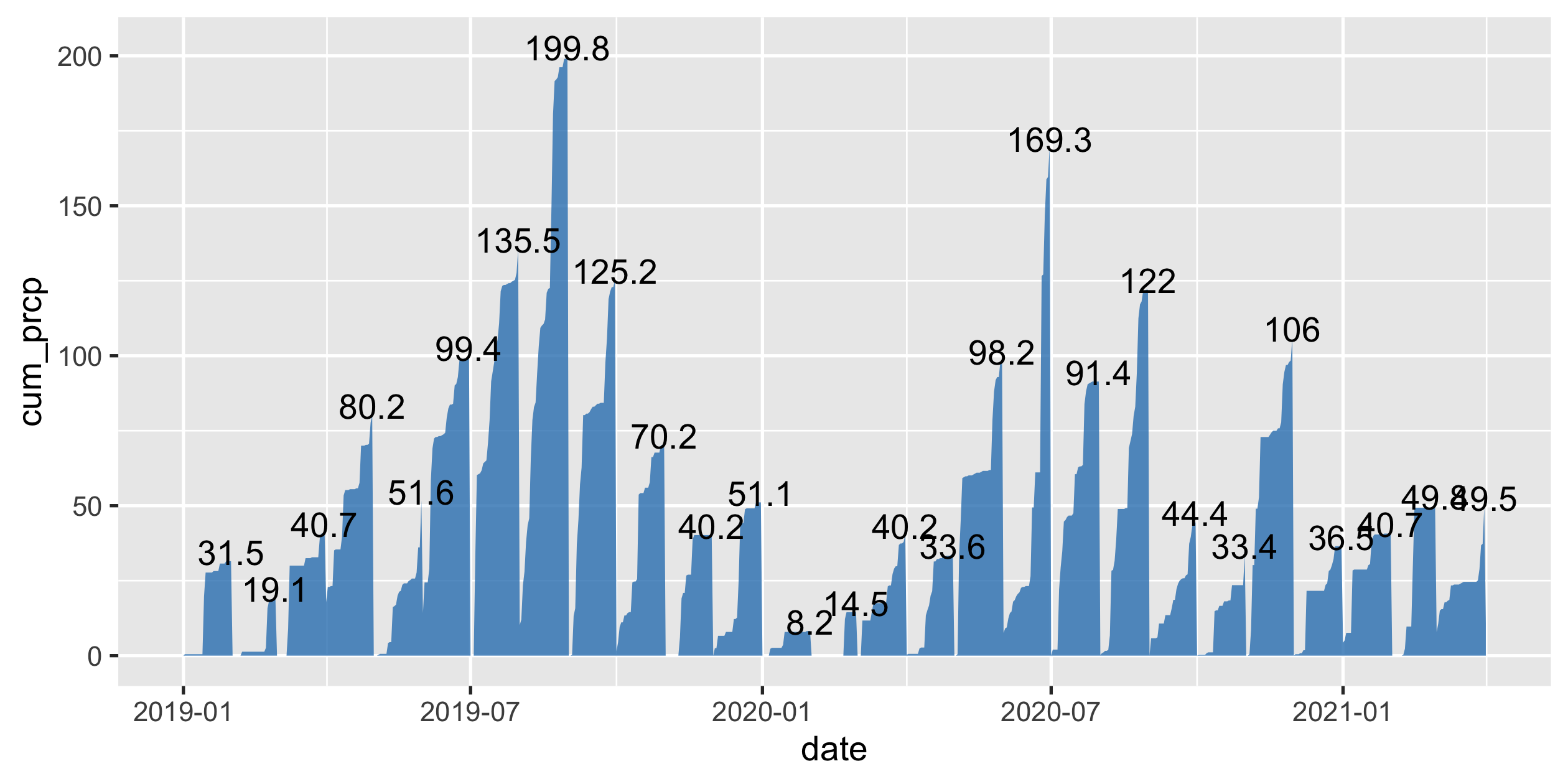
- wrangle

akl_prcp <- aklweather_tidy %>% 
  complete(
    date = full_seq(ymd(c("2019-01-01", "2021-04-01")), 1),
    fill = list(prcp = 0)
  ) %>% 
  group_by(yearmonth = floor_date(date, "1 month")) %>% 
  mutate(cum_prcp = cumsum(prcp)) %>% 
  ungroup()
akl_prcp

#> # A tibble: 822 x 7
#>   date        prcp  tavg  tmax  tmin yearmonth  cum_prcp
#>   <date>     <dbl> <dbl> <dbl> <dbl> <date>        <dbl>
#> 1 2019-01-01   0    20.6  23.2  18.8 2019-01-01      0  
#> 2 2019-01-02   0.5  20.7  23    18.3 2019-01-01      0.5
#> 3 2019-01-03   0    21.1  24.1  18.4 2019-01-01      0.5
#> 4 2019-01-04   0    19.2  22.9  NA   2019-01-01      0.5
#> 5 2019-01-05   0    20    23.3  15   2019-01-01      0.5
#> 6 2019-01-06   0    21.3  23.7  16.9 2019-01-01      0.5
#> # … with 816 more rows

30 / 36

00:30
Your turn

Why do I fill 0 to missing prcp, instead of leaving NA as is?
Why do I calculate monthly cumulative precipitations?


aklweather_tidy %>% 
  complete(date = full_seq(
    ymd(c("2019-01-01", "2021-04-01")), 
    1)) %>% 
  filter(is.na(prcp))

#> # A tibble: 13 x 5
#>    date        prcp  tavg  tmax  tmin
#>    <date>     <dbl> <dbl> <dbl> <dbl>
#>  1 2019-02-16    NA  NA    NA    NA  
#>  2 2019-02-17    NA  NA    NA    NA  
#>  3 2019-02-18    NA  NA    NA    NA  
#>  4 2019-07-01    NA  13.4  18.2  NA  
#>  5 2019-07-02    NA  15.4  17    11.6
#>  6 2019-07-03    NA  16.8  18.2  13.6
#>  7 2019-11-01    NA  14.4  17    12.8
#>  8 2019-11-29    NA  19.7  25.1  NA  
#>  9 2020-04-07    NA  16.9  22.3  NA  
#> 10 2020-10-20    NA  17    NA    NA  
#> 11 2021-02-11    NA  NA    NA    NA  
#> 12 2021-02-12    NA  NA    NA    NA  
#> 13 2021-02-20    NA  NA    NA    NA
31 / 36

Now you need to think why I make this decision not that decision?

- calibrate

- pivot

- rename

- complete

- wrangle

- visualise

Area plot for monthly cumulative rainfall

akl_prcp %>% 
  ggplot(aes(date, cum_prcp)) +
  geom_area(fill = "#3182bd", alpha = 0.8) +
  geom_text(
    aes(label = cum_prcp),
    data = akl_prcp %>% filter(date %in% rollforward(date)),
    nudge_y = 3
  )

32 / 36

felt super try in 2020 summer
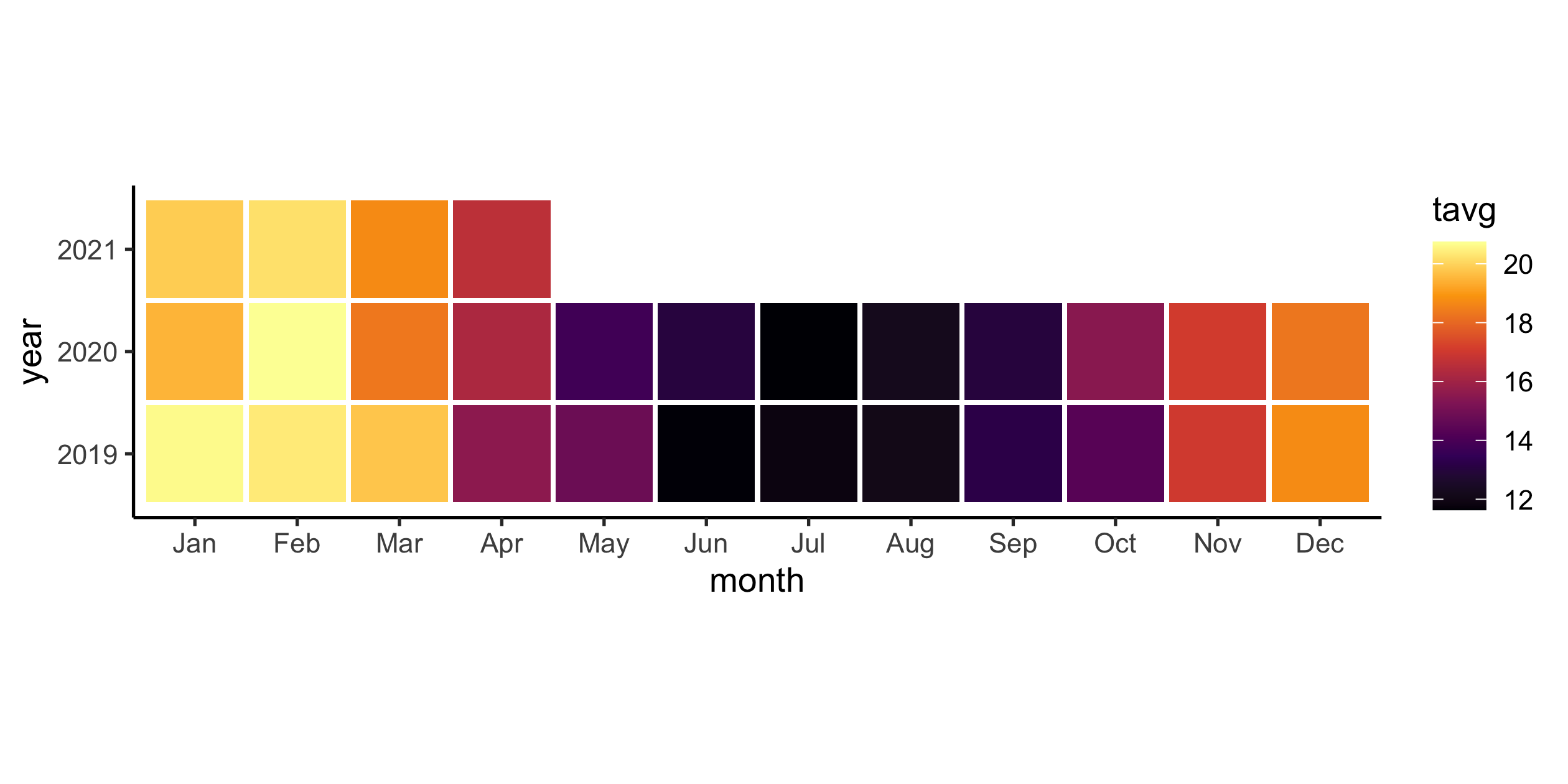
Rainfall in last summer lower than the year before

- calibrate

- pivot

- rename

- complete

- wrangle

akl_monthly_temp <- aklweather_tidy %>% 
  group_by(yearmonth = floor_date(date, "1 month")) %>% 
  summarise(
    tavg = mean(tavg, na.rm = TRUE),
    tmax = mean(tmax, na.rm = TRUE),
    tmin = mean(tmin, na.rm = TRUE)
  )
akl_monthly_temp

#> # A tibble: 28 x 4
#>   yearmonth   tavg  tmax  tmin
#>   <date>     <dbl> <dbl> <dbl>
#> 1 2019-01-01  20.6  24.4 17.3 
#> 2 2019-02-01  20.4  25.2 16.1 
#> 3 2019-03-01  19.7  24.5 15.6 
#> 4 2019-04-01  15.6  20.0 10.5 
#> 5 2019-05-01  14.8  18.9 10.2 
#> 6 2019-06-01  11.7  15.4  7.62
#> # … with 22 more rows

33 / 36

- calibrate

- pivot

- rename

- complete

- wrangle

- visualise

Ribbon plot for monthly temperatures

akl_monthly_temp %>% 
  ggplot(aes(yearmonth, tavg, ymin = tmin, ymax = tmax)) +
  geom_line() +
  geom_ribbon(fill = "#e6550d", alpha = 0.8) +
  scale_x_date(date_labels = "%Y %b")

34 / 36

Why ribbon is missing in the end?

- calibrate

- pivot

- rename

- complete

- wrangle

- visualise

Heatmap for monthly average temperatures

akl_monthly_temp %>% 
  mutate(
    year = year(yearmonth),
    month = month(yearmonth, label = TRUE)) %>% 
  ggplot(aes(month, y = year, fill = tavg)) +
  geom_tile(width = 0.95, height = 0.95) +
  scale_fill_viridis_c(option = "B") +
  coord_fixed() +
  theme_classic()

35 / 36

Reading

36 / 36

Help

Keyboard shortcuts

↑, ←, Pg Up, k

Go to previous slide

↓, →, Pg Dn, Space, j

Go to next slide

Home

Go to first slide

End

Go to last slide

Number + Return

Go to specific slide

b / m / f

Toggle blackout / mirrored / fullscreen mode

Clone slideshow

Toggle presenter mode

Restart the presentation timer

?, h

Toggle this help