STATS 220
R Markdown🧶
1 / 20
- graphics for communication
- keep learning communication
- Rmd: a tool for integrating prose, code, and results
- one md file for multiple documents
+
3 / 20
Rmd: glue 2 things together
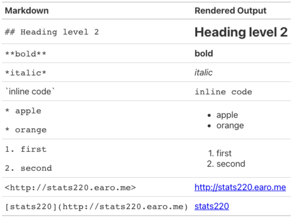
Markdown .md
- Created by John Gruber & Aaron Swartz in 2004
- A lightweight markup language to add formatting elements to plain-text documents, contrasting to WYSIWYG
- Portable, platform independent, everywhere (e.g. Piazza, but not Canvas 😠)

4 / 20
- md originated back to 2004, but emerged around 2010
- aaron, reddit, a loss
- The course website: write in md, and render in html by hugo
- commonmark: it's one of markdown flavours, richer features. e.g. github
- learned it in 5 mins, unlike R
6 / 20
Create R Markdown .Rmd
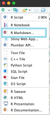
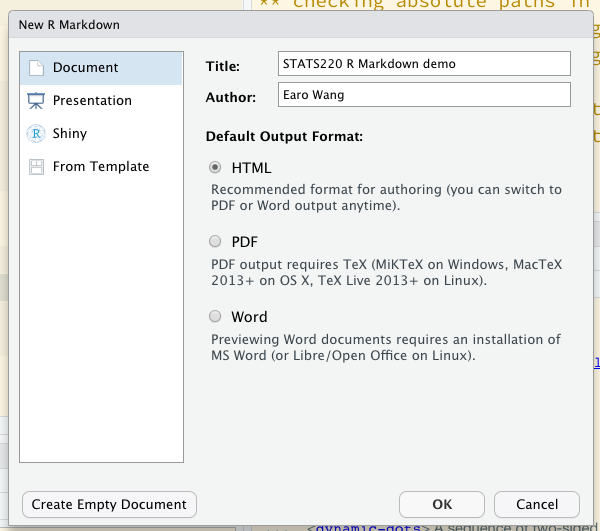
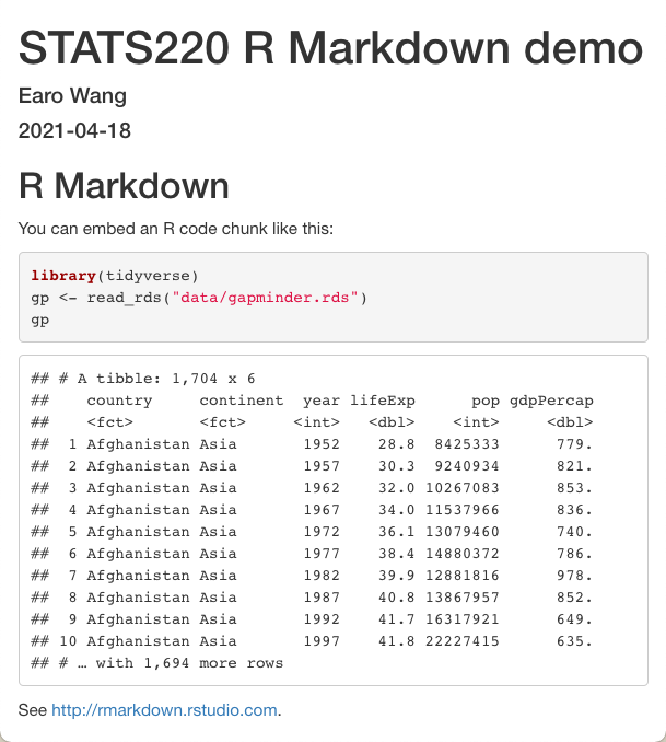
---title: "STATS220 R Markdown demo"author: "Earo Wang"date: "`r lubridate::today()`"output: html_document---```{r setup, include = FALSE}library(knitr)opts_knit$set(root.dir = here::here())opts_chunk$set(echo = TRUE)```## R MarkdownYou can embed an R code chunk like this:```{r gapminder, message = FALSE}library(tidyverse)gp <- read_rds("data/gapminder.rds")gp```See <http://rmarkdown.rstudio.com>.7 / 20
YAML header
YAML is commonly used for configuration files, and starts and ends with
---
`r lubridate::today()`⬆️ inline executable R code
- one markdown file, many formats
pdf_documentxaringan::moon_reader
To compile to PDF,
install.packages('tinytex')tinytex::install_tinytex()---title: "STATS220 R Markdown demo"author: "Earo Wang"date: "`r lubridate::today()`"output: html_document---```{r setup, include = FALSE}library(knitr)opts_knit$set(root.dir = here::here())opts_chunk$set(echo = TRUE)```## R MarkdownYou can embed an R code chunk like this:```{r gapminder, message = FALSE}library(tidyverse)gp <- read_rds("data/gapminder.rds")gp```See <http://rmarkdown.rstudio.com>.8 / 20
R chunk for global settings
```{r setup, include = FALSE}library(knitr)opts_knit$set(root.dir = here::here())opts_chunk$set(echo = TRUE)```⬆️ executable R chunk
r: language enginesetup: unique chunk nameinclude: include chunk output or notecho: display source code or not
---title: "STATS220 R Markdown demo"author: "Earo Wang"date: "`r lubridate::today()`"output: html_document---```{r setup, include = FALSE}library(knitr)opts_knit$set(root.dir = here::here())opts_chunk$set(echo = TRUE)```## R MarkdownYou can embed an R code chunk like this:```{r gapminder, message = FALSE}library(tidyverse)gp <- read_rds("data/gapminder.rds")gp```See <http://rmarkdown.rstudio.com>.9 / 20
Write in markdown
Weave together narrative text and code

---title: "STATS220 R Markdown demo"author: "Earo Wang"date: "`r lubridate::today()`"output: html_document---```{r setup, include = FALSE}library(knitr)opts_knit$set(root.dir = here::here())opts_chunk$set(echo = TRUE)```## R MarkdownYou can embed an R code chunk like this:```{r gapminder, message = FALSE}library(tidyverse)gp <- read_rds("data/gapminder.rds")gp```See <http://rmarkdown.rstudio.com>.10 / 20
R chunk
mpg: unique chunk namemessage: suppress message or not
library(tidyverse)#> ── Attaching packages ─────────────────────────────────────── tidyverse 1.3.1 ──#> ✔ ggplot2 3.3.3 ✔ purrr 0.3.4#> ✔ tibble 3.1.1 ✔ dplyr 1.0.5#> ✔ tidyr 1.1.3 ✔ stringr 1.4.0#> ✔ readr 1.4.0 ✔ forcats 0.5.1#> ── Conflicts ────────────────────────────────────────── tidyverse_conflicts() ──#> ✖ dplyr::filter() masks stats::filter()#> ✖ dplyr::lag() masks stats::lag()---title: "STATS220 R Markdown demo"author: "Earo Wang"date: "`r lubridate::today()`"output: html_document---```{r setup, include = FALSE}library(knitr)opts_knit$set(root.dir = here::here())opts_chunk$set(echo = TRUE)```## R MarkdownYou can embed an R code chunk like this:```{r gapminder, message = FALSE}library(tidyverse)gp <- read_rds("data/gapminder.rds")gp```See <http://rmarkdown.rstudio.com>.11 / 20
Render
3 ways to render an .Rmd
- click

- shortcut: Ctrl/Cmd + Shift + K
rmarkdown::render("demo.Rmd")
12 / 20
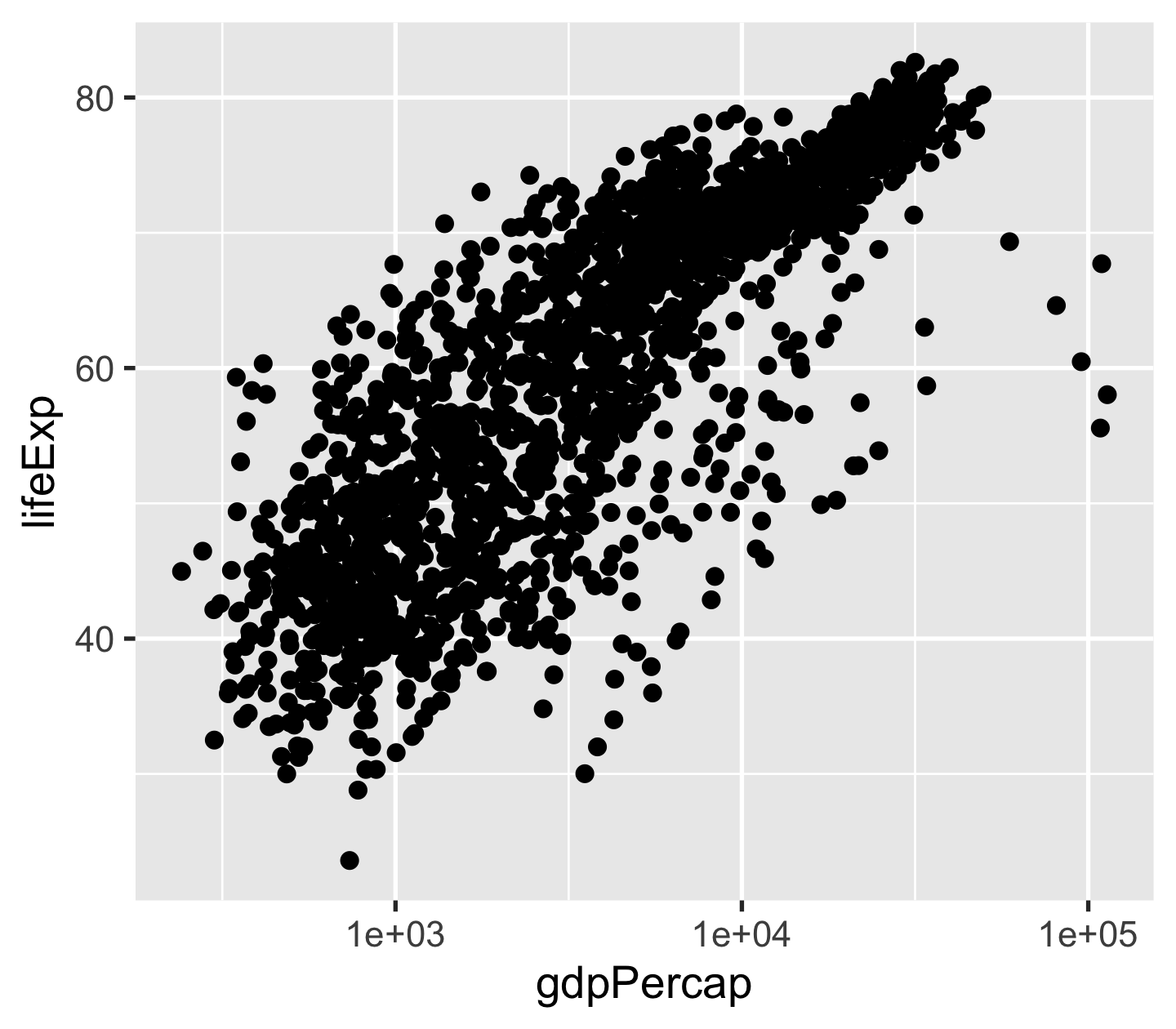
```{r scatterplot, fig.align = "center", fig.width = 4.5, fig.height = 4}ggplot(gp, aes(gdpPercap, lifeExp)) + geom_point() + scale_x_log10()```
13 / 20
```{r scatterplot, fig.align = "center", fig.width = 4.5, fig.height = 4}ggplot(gp, aes(gdpPercap, lifeExp)) + geom_point() + scale_x_log10()```Chunk options
scatterplotgives the chunk a name.fig.align: alignment of figuresfig.width/fig.height- other figure options
Good practice: naming every single chunk!
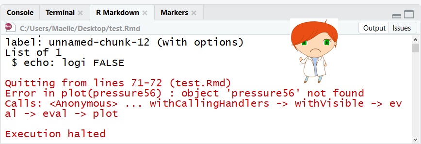
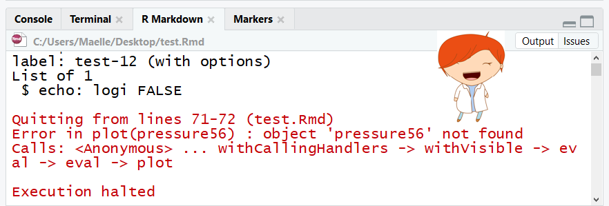
image credit: Maelle Salmon
14 / 20
```{r show-code, ref.label = "scatterplot", eval = FALSE}```Reuse chunks by reference
ref.label: labels of the chunks from which the code of the current chunk is inheritedeval: evaluate the code chunk
Good practice: naming every single chunk!
15 / 20
```{r lm, echo = FALSE, cache = TRUE}fit <- lm(lifeExp ~ log10(gdpPercap), data = gp)kable(coef(summary(fit)))```Chunk options
echo: overwrites the global settingcache: evaluate once and skip for the future
kable() generates a very simple HTML table. ➡️
| Estimate | Std. Error | t value | Pr(>|t|) | |
|---|---|---|---|---|
| (Intercept) | -9.100889 | 1.2276738 | -7.413117 | 0 |
| log10(gdpPercap) | 19.353423 | 0.3425372 | 56.500206 | 0 |
16 / 20
Beyond : language engines
```{python hello}# remotes::install_github("rstudio/reticulate")x = "hello, python world!"print(x.split(" "))```#> ['hello,', 'python', 'world!']```{sh head}head -4 data/pisa/pisa-student.csv```#> year,country,school_id,student_id,mother_educ,father_educ,gender,computer,internet,math,read,science,stu_wgt,desk,room,dishwasher,television,computer_n,car,book,wealth,escs#> 2000,ALB,1001,1,NA,NA,female,NA,no,324.35,397.87,345.66,2.16,yes,no,no,1,3+,1,11-50,-0.6,0.10575582991490981#> 2000,ALB,1001,3,NA,NA,female,NA,no,NA,368.41,385.83,2.16,yes,yes,no,2,0,0,1-10,-1.84,-1.424044581128788#> 2000,ALB,1001,6,NA,NA,male,NA,no,NA,294.17,327.94,2.16,yes,yes,no,2,0,0,1-10,-1.46,-1.30668385536561217 / 20
Beyond : language engines
```{r db}library(RSQLite)db <- dbConnect(SQLite(), dbname = "data/pisa/pisa-student.db")``````{sql query, connection = db, output.var = "pisa18"}SELECT * FROM pisa WHERE year = 2018```#> # A tibble: 612,004 x 22#> year country school_id student_id mother_educ father_educ#> <dbl> <chr> <chr> <chr> <chr> <chr> #> 1 2018 ALB 800002 800251 ISCED 3A ISCED 3A #> 2 2018 ALB 800002 800402 ISCED 2 ISCED 2 #> 3 2018 ALB 800002 801902 ISCED 2 ISCED 2 #> 4 2018 ALB 800002 803546 ISCED 2 ISCED 2 #> 5 2018 ALB 800002 804776 ISCED 2 ISCED 3A #> 6 2018 ALB 800002 804825 ISCED 2 ISCED 2 #> # … with 611,998 more rows, and 16 more variables:#> # gender <chr>, computer <chr>, internet <chr>,#> # math <dbl>, read <dbl>, science <dbl>, stu_wgt <dbl>,#> # desk <chr>, room <chr>, dishwasher <chr>,#> # television <chr>, computer_n <chr>, car <chr>,#> # book <chr>, wealth <dbl>, escs <dbl>18 / 20
Beyond : language engines
names(knitr::knit_engines$get())#> [1] "awk" "bash" "coffee" "gawk" "groovy" "haskell" #> [7] "lein" "mysql" "node" "octave" "perl" "psql" #> [13] "Rscript" "ruby" "sas" "scala" "sed" "sh" #> [19] "stata" "zsh" "highlight" "Rcpp" "tikz" "dot" #> [25] "c" "cc" "fortran" "fortran95" "asy" "cat" #> [31] "asis" "stan" "block" "block2" "js" "css" #> [37] "sql" "go" "python" "julia" "sass" "scss" #> [43] "R" "bslib"19 / 20
