


Dynamic documents
- Combine code, rendered output (such as figures), and prose
- Reproduce your analyses
- Collaborate and share code with others
- Communicate your results with others
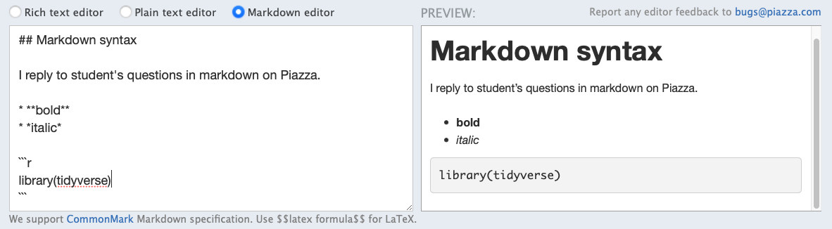
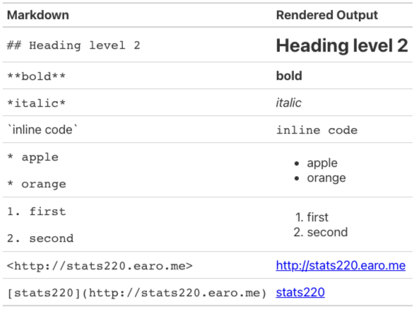
Markdown .md
- Created by John Gruber & Aaron Swartz in 2004
- A lightweight markup language to add formatting elements to plain-text documents, contrasting to WYSIWYG
- Portable, platform independent, everywhere (e.g. Piazza, but not Canvas 😠)
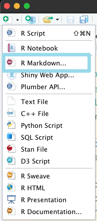
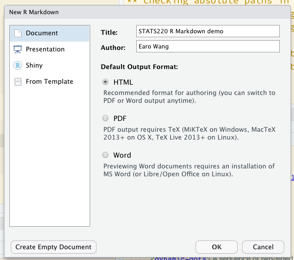
Create R Markdown .Rmd
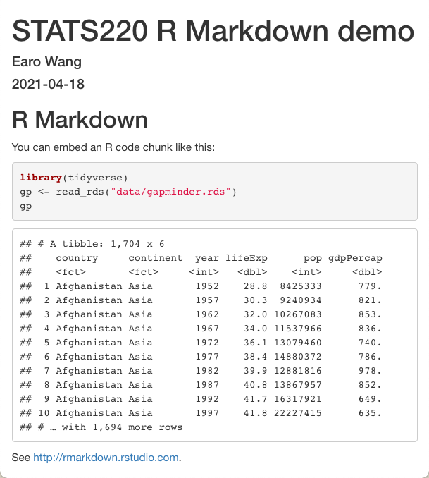
---title: "STATS220 R Markdown demo"author: "Earo Wang"date: "`r lubridate::today()`"output: html_document---```{r setup, include = FALSE}library(knitr)opts_knit$set(root.dir = here::here())opts_chunk$set(echo = TRUE)```## R MarkdownYou can embed an R code chunk like this:```{r gapminder, message = FALSE}library(tidyverse)gp <- read_rds("data/gapminder.rds")gp```See <http://rmarkdown.rstudio.com>.Write in markdown
Weave together narrative text and code

---title: "STATS220 R Markdown demo"author: "Earo Wang"date: "`r lubridate::today()`"output: html_document---```{r setup, include = FALSE}library(knitr)opts_knit$set(root.dir = here::here())opts_chunk$set(echo = TRUE)```## R MarkdownYou can embed an R code chunk like this:```{r gapminder, message = FALSE}library(tidyverse)gp <- read_rds("data/gapminder.rds")gp```See <http://rmarkdown.rstudio.com>.Render
3 ways to render an .Rmd
- click

- shortcut: Ctrl/Cmd + Shift + K
rmarkdown::render("demo.Rmd")
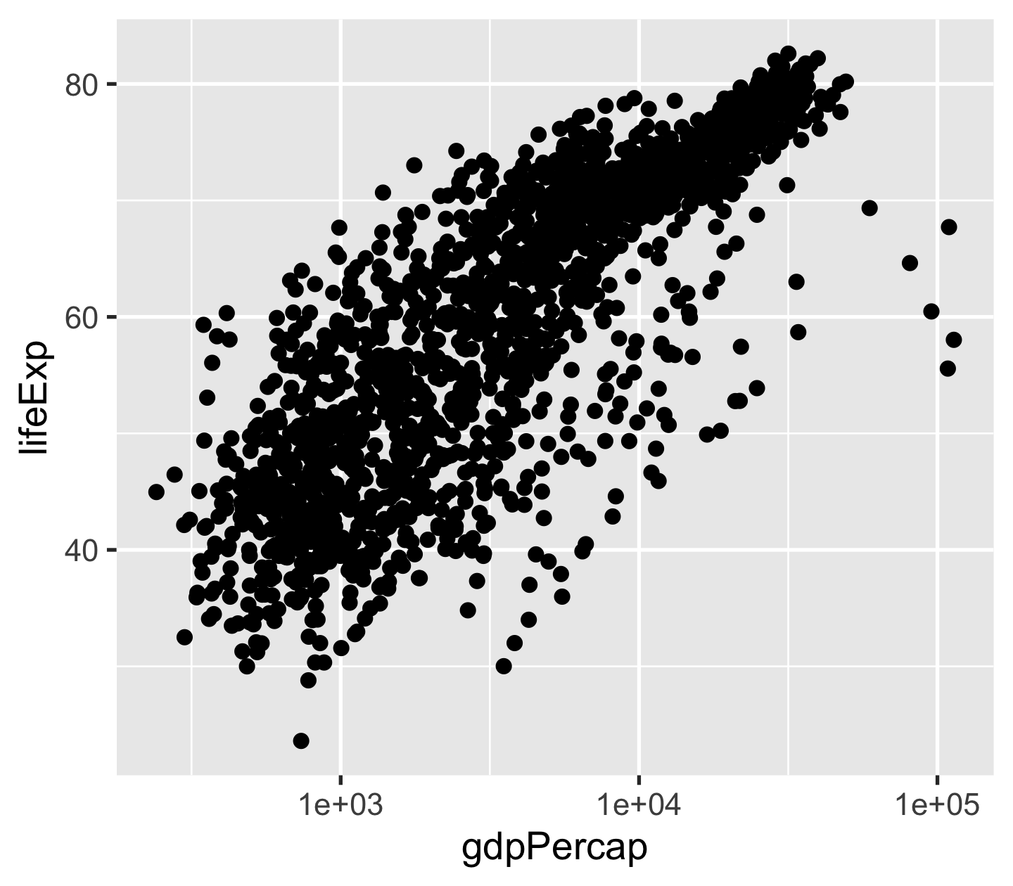
```{r scatterplot, fig.align = "center", fig.width = 4.5, fig.height = 4}ggplot(gp, aes(gdpPercap, lifeExp)) + geom_point() + scale_x_log10()```
```{r scatterplot, fig.align = "center", fig.width = 4.5, fig.height = 4}ggplot(gp, aes(gdpPercap, lifeExp)) + geom_point() + scale_x_log10()```Chunk options
scatterplotgives the chunk a name.fig.align: alignment of figuresfig.width/fig.height- other figure options
Good practice: naming every single chunk!
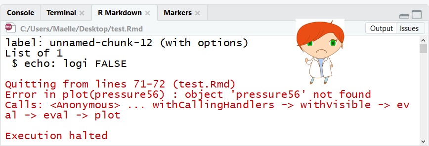
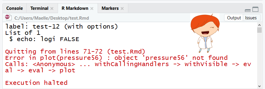
image credit: Maelle Salmon
```{r show-code, ref.label = "scatterplot", eval = FALSE}```Reuse chunks by reference
ref.label: labels of the chunks from which the code of the current chunk is inheritedeval: evaluate the code chunk
Good practice: naming every single chunk!