Lab 05

This lab exercise is due 23:59 Monday 26 April (NZST).

• You should submit an R file (i.e. file extension .R) containing R code that assigns the appropriate values to the appropriate symbols.
• Your R file will be executed in order and checked against the values that have been assigned to the symbols using an automatic grading system. Marks will be fully deducted for non-identical results.
• Intermediate steps to achieve the final results will NOT be checked.
• Each question is worth 0.2 points.
• You should submit your R file on Canvas.
• Late assignments are NOT accepted unless prior arrangement for medical/compassionate reasons.

In this lab exercise, you are going to work with two data sets: step-count.csv that contains Dr Wang’s hourly step counts, and location.csv with cities where she was in 2019. You shall use the following code snippet (and include them upfront in your R file) to start with this lab session:

library(lubridate)
library(tidyverse)
step_count_raw <- read_csv("data/step-count/step-count.csv",
  locale = locale(tz = "Australia/Melbourne"))
location <- read_csv("data/step-count/location.csv")
step_count <- step_count_raw %>% 
  rename_with(~ c("date_time", "date", "count")) %>% 
  left_join(location) %>% 
  mutate(location = replace_na(location, "Melbourne"))
step_count

#> # A tibble: 5,448 x 4
#>    date_time           date       count location 
#>    <dttm>              <date>     <dbl> <chr>    
#>  1 2019-01-01 09:00:00 2019-01-01   764 Melbourne
#>  2 2019-01-01 10:00:00 2019-01-01   913 Melbourne
#>  3 2019-01-02 00:00:00 2019-01-02     9 Melbourne
#>  4 2019-01-02 10:00:00 2019-01-02  2910 Melbourne
#>  5 2019-01-02 11:00:00 2019-01-02  1390 Melbourne
#>  6 2019-01-02 12:00:00 2019-01-02  1020 Melbourne
#>  7 2019-01-02 13:00:00 2019-01-02   472 Melbourne
#>  8 2019-01-02 15:00:00 2019-01-02  1220 Melbourne
#>  9 2019-01-02 16:00:00 2019-01-02  1670 Melbourne
#> 10 2019-01-02 17:00:00 2019-01-02  1390 Melbourne
#> # … with 5,438 more rows

Suppose that you have created an Rproj for this course. You need to download step-count.csv here and location.csv here, to data/step-count/ under your Rproj folder.

• You’re required to use relative file paths data/step-count/step-count.csv and data/step-count/location.csv to import these data. NO marks will be given to this lab for using URL links or different file paths.
• NO marks given to the question, in which you apply theme() and aesthetics other than what I instruct to the plot.

Question 1

Calculate average daily step counts for every location, from step_count.

You should end up with a tibble called city_avg_steps.

city_avg_steps

#> # A tibble: 4 x 2
#>   location      avg_count
#>   <chr>             <dbl>
#> 1 Austin            7738.
#> 2 Denver           12738.
#> 3 Melbourne         7912.
#> 4 San Francisco    13990.

Question 2

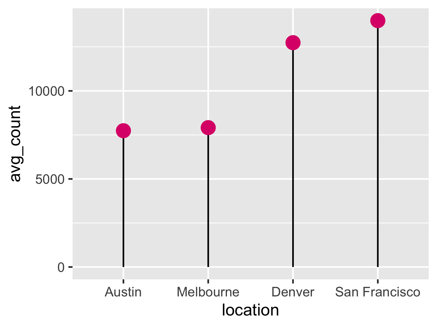
Create a lollipop plot to display average daily steps at each location from low to high.

You should end up with a ggplot called p1, with

• point: size = 4 and colour = "#dd1c77".

p1

Question 3

Add two new columns to the step_count:

1. time: hour of the day in factor.
2. country: when location is Melbourne, set values with "AU"; otherwise "US".

You should end up with a tibble called step_count_time.

step_count_time

#> # A tibble: 5,448 x 6
#>    date_time           date       count location  time  country
#>    <dttm>              <date>     <dbl> <chr>     <fct> <chr>  
#>  1 2019-01-01 09:00:00 2019-01-01   764 Melbourne 9     AU     
#>  2 2019-01-01 10:00:00 2019-01-01   913 Melbourne 10    AU     
#>  3 2019-01-02 00:00:00 2019-01-02     9 Melbourne 0     AU     
#>  4 2019-01-02 10:00:00 2019-01-02  2910 Melbourne 10    AU     
#>  5 2019-01-02 11:00:00 2019-01-02  1390 Melbourne 11    AU     
#>  6 2019-01-02 12:00:00 2019-01-02  1020 Melbourne 12    AU     
#>  7 2019-01-02 13:00:00 2019-01-02   472 Melbourne 13    AU     
#>  8 2019-01-02 15:00:00 2019-01-02  1220 Melbourne 15    AU     
#>  9 2019-01-02 16:00:00 2019-01-02  1670 Melbourne 16    AU     
#> 10 2019-01-02 17:00:00 2019-01-02  1390 Melbourne 17    AU     
#> # … with 5,438 more rows

levels(step_count_time$time)

#>  [1] "0"  "1"  "2"  "3"  "4"  "5"  "6"  "7"  "8"  "9"  "10" "11" "12"
#> [14] "13" "14" "15" "16" "17" "18" "19" "20" "21" "22" "23"

step_count_time %>% 
  filter(country == "US")

#> # A tibble: 323 x 6
#>    date_time           date       count location time  country
#>    <dttm>              <date>     <dbl> <chr>    <fct> <chr>  
#>  1 2019-01-15 03:00:00 2019-01-15     8 Austin   3     US     
#>  2 2019-01-15 05:00:00 2019-01-15   355 Austin   5     US     
#>  3 2019-01-15 06:00:00 2019-01-15  1800 Austin   6     US     
#>  4 2019-01-15 07:00:00 2019-01-15   261 Austin   7     US     
#>  5 2019-01-15 11:00:00 2019-01-15  1240 Austin   11    US     
#>  6 2019-01-15 12:00:00 2019-01-15   795 Austin   12    US     
#>  7 2019-01-15 13:00:00 2019-01-15   206 Austin   13    US     
#>  8 2019-01-15 14:00:00 2019-01-15   481 Austin   14    US     
#>  9 2019-01-16 01:00:00 2019-01-16  2220 Austin   1     US     
#> 10 2019-01-16 02:00:00 2019-01-16   711 Austin   2     US     
#> # … with 313 more rows

Question 4

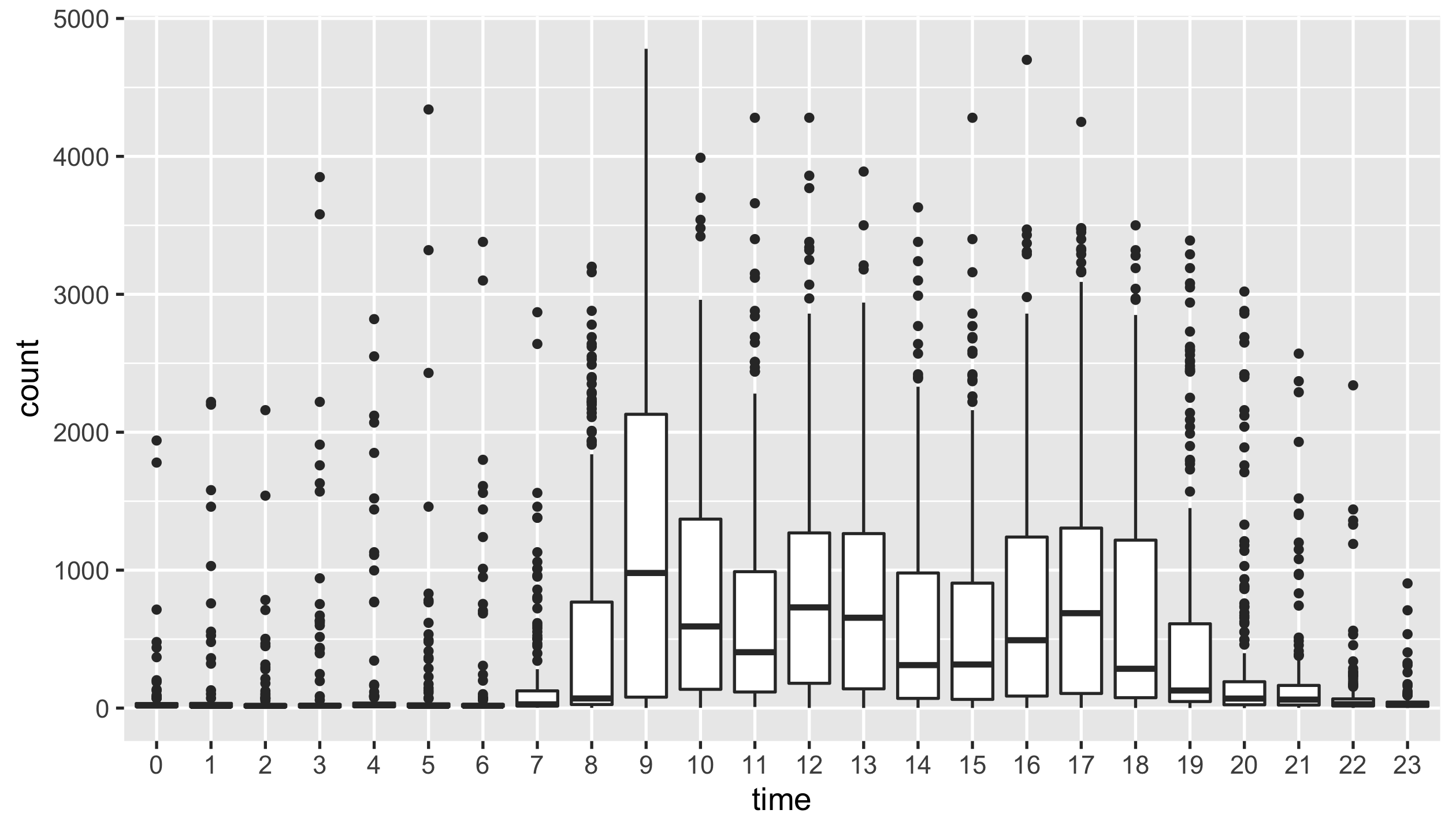
Create a boxplot that visualises the distribution of hourly step counts.

You should end up with a ggplot called p2, with outlier.size = 1.

p2

Question 5

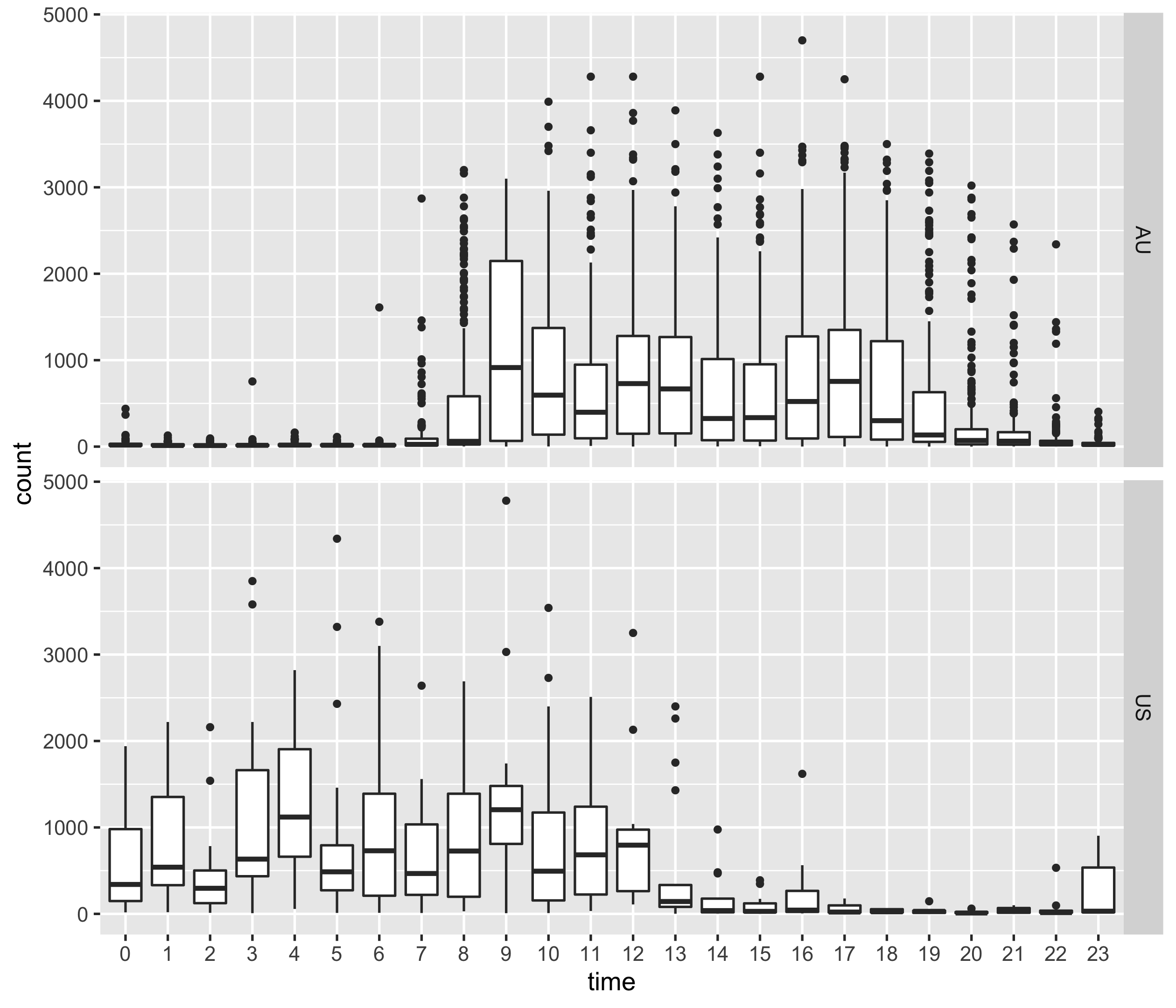
Facet p2 by countries on rows.

You should end up with a ggplot called p3, with outlier.size = 1.

p3

Question4fun (NO marks)

This is a challenging question, where you need to have solid understanding about time zones in R.

Your instructor wanders like a ghost during night times in US, due to time zone issues. To correct these spooky behaviours, time zones have to be adjusted to the local time zone.

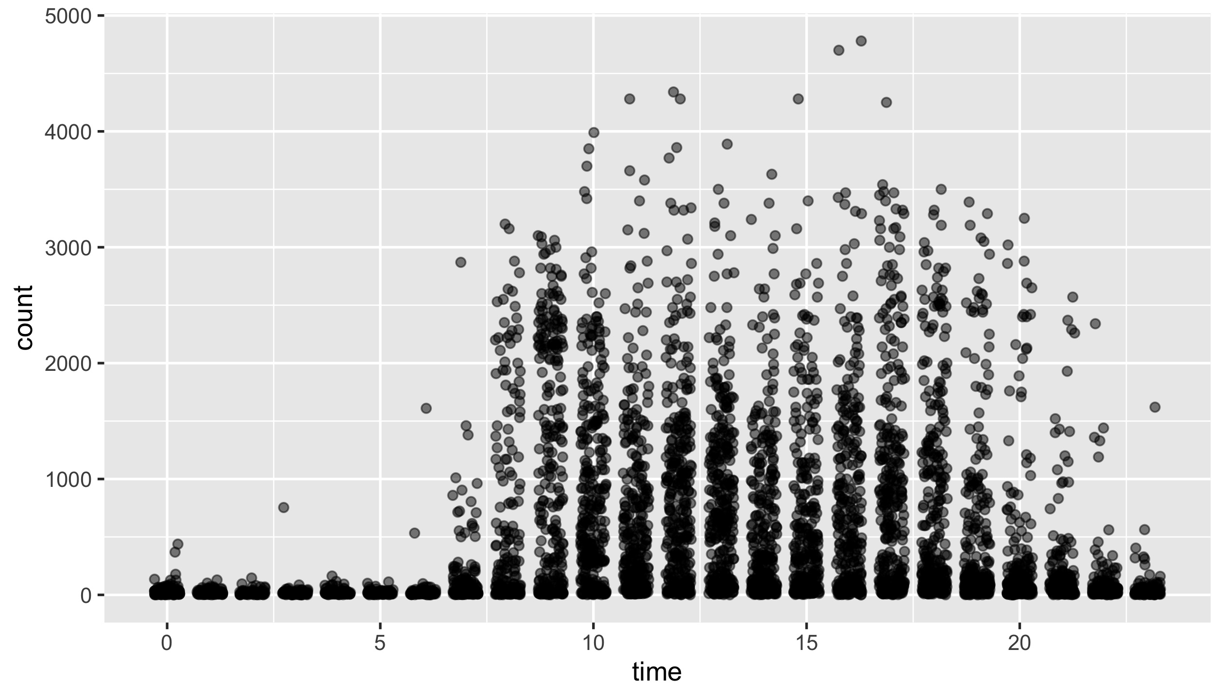
Create a jitter plot to demonstrate the corrected hourly step counts, with

• position = position_jitter(0.3, seed = 220) and alpha = 0.5