Lab 10 Solution
This lab exercise is due 23:59 Monday 31 May (NZST).
- You should submit an R file (i.e. file extension
.R) containing R code that assigns the appropriate values to the appropriate symbols. - Your R file will be executed in order and checked against the values that have been assigned to the symbols using an automatic grading system. Marks will be fully deducted for non-identical results.
- Intermediate steps to achieve the final results will NOT be checked.
- Each question is worth 0.2 points.
- You should submit your R file on Canvas.
- Late assignments are NOT accepted unless prior arrangement for medical/compassionate reasons.
In this lab exercise, you are going to carry out sentiment analysis from the critics for Animal Crossing - New Horizons. You shall use the following code snippet (and include them upfront in your R file) for this lab session:
library(ggrepel)
library(tidytext)
library(tidyverse)
rm_words <- c("animal", "crossing", "horizons", "game", "nintendo",
  "switch", "series", "island")
critic <- read_tsv("data/animal-crossing/critic.tsv")
critic
#> # A tibble: 107 x 4
#>    grade publication    text                                date
#>    <dbl> <chr>          <chr>                               <date>
#>  1   100 Pocket Gamer … Animal Crossing; New Horizons, muc… 2020-03-16
#>  2   100 Forbes         Know that if you’re overwhelmed wi… 2020-03-16
#>  3   100 Telegraph      With a game this broad and lengthy… 2020-03-16
#>  4   100 VG247          Animal Crossing: New Horizons is e… 2020-03-16
#>  5   100 Nintendo Insi… Above all else, Animal Crossing: N… 2020-03-16
#>  6   100 Trusted Revie… Animal Crossing: New Horizons is t… 2020-03-16
#>  7   100 VGC            Nintendo's comforting life sim is … 2020-03-16
#>  8   100 God is a Geek  A beautiful, welcoming game that i… 2020-03-16
#>  9   100 Nintendo Life  Animal Crossing: New Horizons take… 2020-03-16
#> 10   100 Daily Star     Similar to how Breath of the Wild … 2020-03-16
#> # … with 97 more rows
Suppose that you have created an Rproj for this course. You need to
download critic.tsv
here
to data/animal-crossing/ under your Rproj folder.
- You’re required to use relative file paths
data/animal-crossing/critic.tsvto import these data. NO marks will be given to this lab for using URL links or different file paths.
Question 1
Tokenise the text column from critic into the word column as
one-word-per-row.
You should end up with a tibble called critic_tokens.
critic_tokens <- critic %>%
  unnest_tokens(output = word, input = text)
critic_tokens
#> # A tibble: 5,741 x 4
#>    grade publication     date       word
#>    <dbl> <chr>           <date>     <chr>
#>  1   100 Pocket Gamer UK 2020-03-16 animal
#>  2   100 Pocket Gamer UK 2020-03-16 crossing
#>  3   100 Pocket Gamer UK 2020-03-16 new
#>  4   100 Pocket Gamer UK 2020-03-16 horizons
#>  5   100 Pocket Gamer UK 2020-03-16 much
#>  6   100 Pocket Gamer UK 2020-03-16 like
#>  7   100 Pocket Gamer UK 2020-03-16 its
#>  8   100 Pocket Gamer UK 2020-03-16 predecessors
#>  9   100 Pocket Gamer UK 2020-03-16 operates
#> 10   100 Pocket Gamer UK 2020-03-16 outside
#> # … with 5,731 more rows
Question 2
Remove stop words (using the "smart" source) from critic_tokens.
You should end up with a tibble called critic_smart.
critic_smart <- critic_tokens %>%
  anti_join(get_stopwords(source = "smart"))
critic_smart
#> # A tibble: 2,469 x 4
#>    grade publication     date       word
#>    <dbl> <chr>           <date>     <chr>
#>  1   100 Pocket Gamer UK 2020-03-16 animal
#>  2   100 Pocket Gamer UK 2020-03-16 crossing
#>  3   100 Pocket Gamer UK 2020-03-16 horizons
#>  4   100 Pocket Gamer UK 2020-03-16 predecessors
#>  5   100 Pocket Gamer UK 2020-03-16 operates
#>  6   100 Pocket Gamer UK 2020-03-16 boundaries
#>  7   100 Pocket Gamer UK 2020-03-16 games
#>  8   100 Pocket Gamer UK 2020-03-16 tension
#>  9   100 Pocket Gamer UK 2020-03-16 feel
#> 10   100 Pocket Gamer UK 2020-03-16 sprinting
#> # … with 2,459 more rows
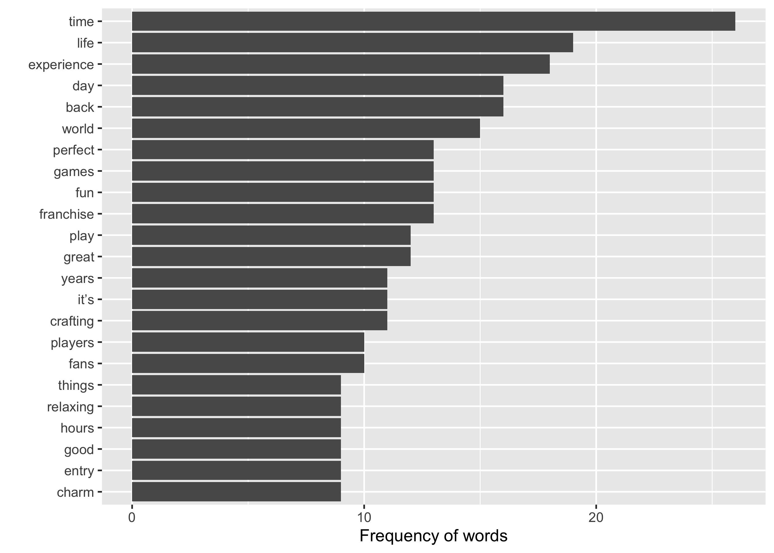
Question 3
Filter out these common words (specified in rm_words) from
critic_smart, and create a bar chart to display the top 20 most common
words.
You should end up with a ggplot called p1, with labels:
- x:
"Frequency of words" - y:
""
p1 <- critic_smart %>%
  count(word) %>%
  filter(!word %in% rm_words) %>%
  slice_max(n, n = 20) %>%
  ggplot(aes(x = n, y = fct_reorder(word, n))) +
  geom_col() +
  labs(x = "Frequency of words", y = "")
p1
Question 4
To summarise the sentiments of critic_smart, you need to:
- join
critic_smartwith the sentiment lexicon sourced from"bing" - count the frequency of
sentimentandword - arrange the frequency of words in ascending order
You should end up with a tibble called critic_sentiments.
critic_sentiments <- critic_smart %>%
  inner_join(get_sentiments("bing")) %>%
  count(sentiment, word) %>%
  arrange(n)
critic_sentiments
#> # A tibble: 234 x 3
#>    sentiment word          n
#>    <chr>     <chr>     <int>
#>  1 negative  addicted      1
#>  2 negative  addicting     1
#>  3 negative  annoyance     1
#>  4 negative  archaic       1
#>  5 negative  betraying     1
#>  6 negative  bore          1
#>  7 negative  bored         1
#>  8 negative  boring        1
#>  9 negative  break         1
#> 10 negative  burden        1
#> # … with 224 more rows
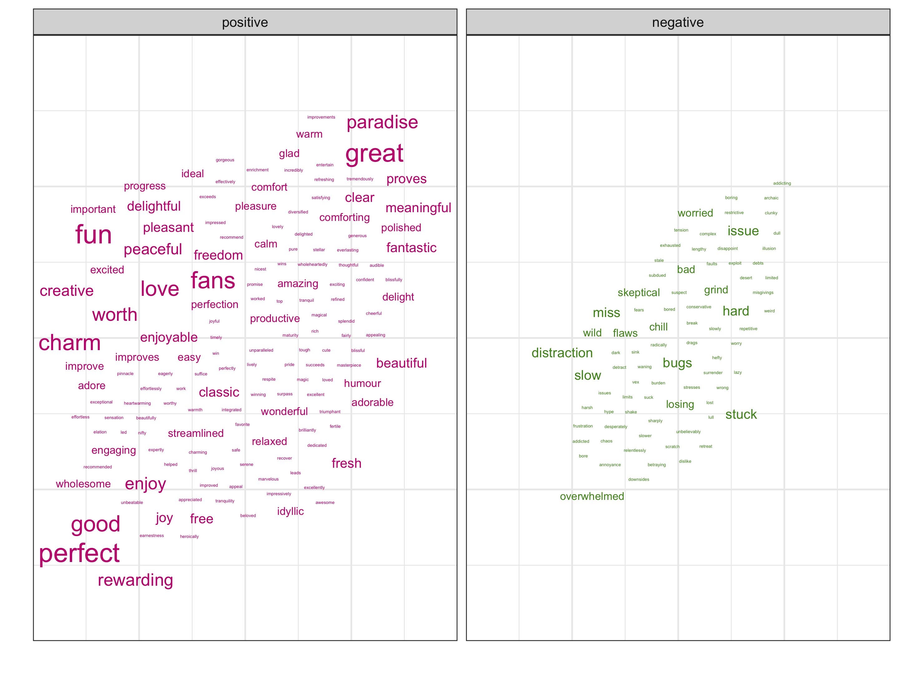
Question 5
Create a small multiple of wordclouds for critic_sentiments,
conditional on the sentiment column.
- Use
geom_text_repel()from {ggrepel} to label each word, sized by the frequency of words and coloured bysentiment. - Set the common origin
aes(x = 0, y = 0)and letgeom_text_repel()pull words away from the origin, since no coordinates are provided to each word in wordcloud. - Supply
geom_text_repel()with the following arguments:force_pull = 0max.overlaps = Infsegment.color = NApoint.padding = NAseed = 220
- Map
"#c51b7d"to positive sentiments, and"#4d9221"to negative ones.
You should end up with a ggplot called p2, with
- the black-and-white theme
- axes ticks, texts, and labels removed
- legends removed
NOTE: if your placement of words is slightly off from the sample plot, that’s okay, since the figure size affects the placement.
p2 <- critic_sentiments %>%
  mutate(sentiment = fct_rev(sentiment)) %>%
  ggplot(aes(x = 0, y = 0)) +
  geom_text_repel(aes(label = word, size = n, colour = sentiment),
    force_pull = 0, max.overlaps = Inf,
    segment.color = NA, point.padding = NA, seed = 220) +
  facet_grid(~ sentiment) +
  scale_colour_manual(values = c("#c51b7d", "#4d9221")) +
  guides(colour = FALSE, size = FALSE) +
  theme_bw() +
  theme(axis.text = element_blank(), axis.ticks = element_blank()) +
  labs(x = "", y = "")
p2