STATS 220
Data import⬇️/export⬆️
Atomic vector (1d)
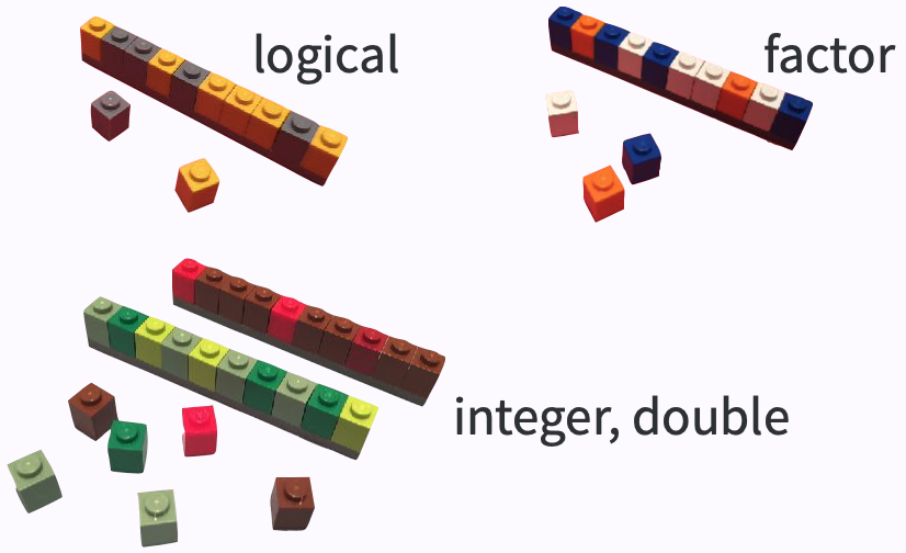
dept <- c("Physics", "Mathematics", "Statistics", "Computer Science")nstaff <- c(12L, 8L, 20L, 23L)image credit: Jenny Bryan
- an ensemble of scalars -> vectors
1d ➡️ 2d

library(tibble)sci_tbl <- tibble( department = dept, count = nstaff, percentage = count / sum(count))sci_tbl#> # A tibble: 4 x 3#> department count percentage#> <chr> <int> <dbl>#> 1 Physics 12 0.190#> 2 Mathematics 8 0.127#> 3 Statistics 20 0.317#> 4 Computer Science 23 0.365image credit: Jenny Bryan
- an ensemble of vectors -> rect data/tabular data, like spreadsheet
Beyond 1d vectors
1. Lists
2. Matrices and arrays
3. Data frames and tibbles
- Common data strs beyond 1d
- start with the most flex one
- briefly talk about mat
- focus on data frames, more specifically tibbles
data strs
- lists
An object contains elements of different data types.
lst <- list( # list constructor/creator 1:3, "a", c(TRUE, FALSE, TRUE), c(2.3, 5.9))lst#> [[1]]#> [1] 1 2 3#> #> [[2]]#> [1] "a"#> #> [[3]]#> [1] TRUE FALSE TRUE#> #> [[4]]#> [1] 2.3 5.9- to create a list using
list() - put 4 atomic vectors inside my lst
- a list of 4 elements, or length of 4
data strs
- lists

data type
typeof(lst) # primitive type#> [1] "list"data class
class(lst) # type + attributes#> [1] "list"data structure
str(lst)# el can be of diff lengths#> List of 4#> $ : int [1:3] 1 2 3#> $ : chr "a"#> $ : logi [1:3] TRUE FALSE TRUE#> $ : num [1:2] 2.3 5.9- vis rep: a container, 4 items inside
- primitive: original, cannot be modified
- class: type + attrs, can be modified
- rstudio values uses
str()
data strs
- lists
lst#> [[1]]#> [1] 1 2 3#> #> [[2]]#> [1] "a"#> #> [[3]]#> [1] TRUE FALSE TRUE#> #> [[4]]#> [1] 2.3 5.9
data strs
- lists
A list can contain other lists, i.e. recursive
# a named liststr(list(first_el = lst, second_el = mtcars))#> List of 2#> $ first_el :List of 4#> ..$ : int [1:3] 1 2 3#> ..$ : chr "a"#> ..$ : logi [1:3] TRUE FALSE TRUE#> ..$ : num [1:2] 2.3 5.9#> $ second_el:'data.frame': 32 obs. of 11 variables:#> ..$ mpg : num [1:32] 21 21 22.8 21.4 18.7 18.1 14.3 24.4 22.8 19.2 ...#> ..$ cyl : num [1:32] 6 6 4 6 8 6 8 4 4 6 ...#> ..$ disp: num [1:32] 160 160 108 258 360 ...#> ..$ hp : num [1:32] 110 110 93 110 175 105 245 62 95 123 ...#> ..$ drat: num [1:32] 3.9 3.9 3.85 3.08 3.15 2.76 3.21 3.69 3.92 3.92 ...#> ..$ wt : num [1:32] 2.62 2.88 2.32 3.21 3.44 ...#> ..$ qsec: num [1:32] 16.5 17 18.6 19.4 17 ...#> ..$ vs : num [1:32] 0 0 1 1 0 1 0 1 1 1 ...#> ..$ am : num [1:32] 1 1 1 0 0 0 0 0 0 0 ...#> ..$ gear: num [1:32] 4 4 4 3 3 3 3 4 4 4 ...#> ..$ carb: num [1:32] 4 4 1 1 2 1 4 2 2 4 ...- most flex: put a list into a list
- a named list
data strs
- lists
Test for a list
is.list(lst)#> [1] TRUECoerce to a list
as.list(1:3)#> [[1]]#> [1] 1#> #> [[2]]#> [1] 2#> #> [[3]]#> [1] 3- to test if an object is one type, funs prefixed
is - to coerce/convert from one type to another type, funs prefixed with
as - from a vector of integers to a list
data strs
- lists
Subset by []
lst[1]#> [[1]]#> [1] 1 2 3Subset by [[]]
lst[[1]]#> [1] 1 2 3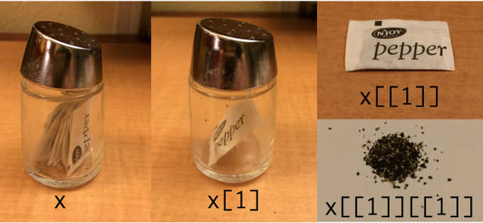
image credit: Hadley Wickham
data strs
- lists
- matrices
2D structure of homogeneous data types
matrix()to construct a matrix
matrix(1:9, nrow = 3)#> [,1] [,2] [,3]#> [1,] 1 4 7#> [2,] 2 5 8#> [3,] 3 6 9as.matrix()to coerce to a matrixis.matrix()to test for a matrix
- we don't deal with matrix in 220, matrix for computational stats.
data strs
- lists
- matrices
array: more than 2D matrix
array(1:9, dim = c(1, 3, 3))#> , , 1#> #> [,1] [,2] [,3]#> [1,] 1 2 3#> #> , , 2#> #> [,1] [,2] [,3]#> [1,] 4 5 6#> #> , , 3#> #> [,1] [,2] [,3]#> [1,] 7 8 9data strs
- lists
- matrices
- tibbles
A data frame is a named list of vectors of the same length.
sci_df <- data.frame( department = dept, count = nstaff)sci_df#> department count#> 1 Physics 12#> 2 Mathematics 8#> 3 Statistics 20#> 4 Computer Science 23data strs
- lists
- matrices
- tibbles
The underlying data type is a list.
typeof(sci_df)#> [1] "list"data class
class(sci_df)#> [1] "data.frame"data attributes (meta info)
attributes(sci_df)#> $names#> [1] "department" "count" #> #> $class#> [1] "data.frame"#> #> $row.names#> [1] 1 2 3 4data.framerepresents tabular data in R- attributes: colnames and rownames
data strs
- lists
- matrices
- tibbles
A tibble is a modern reimagining of the data frame.
library(tibble)sci_tbl <- tibble( department = dept, count = nstaff, percentage = count / sum(count))sci_tbl#> # A tibble: 4 x 3#> department count percentage#> <chr> <int> <dbl>#> 1 Physics 12 0.190#> 2 Mathematics 8 0.127#> 3 Statistics 20 0.317#> 4 Computer Science 23 0.365as_tibble()to coerce to a tibbleis_tibble()to test for a tibble
- why we call it
tibble
data strs
- lists
- matrices
- tibbles
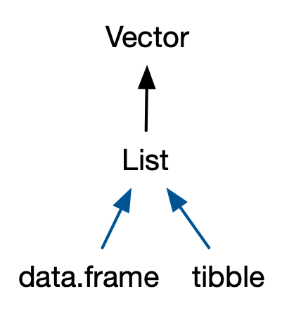
typeof(sci_tbl) # list in essence#> [1] "list"class(sci_tbl) # tibble is a special class of data.frame#> [1] "tbl_df" "tbl" "data.frame"- multi cls: left to right, specific to more general
Why tibble not data frame?
sci_df <- data.frame( department = dept, count = nstaff)sci_df#> department count#> 1 Physics 12#> 2 Mathematics 8#> 3 Statistics 20#> 4 Computer Science 23sci_tbl <- tibble( department = dept, count = nstaff, percentage = count / sum(count))sci_tbl#> # A tibble: 4 x 3#> department count percentage#> <chr> <int> <dbl>#> 1 Physics 12 0.190#> 2 Mathematics 8 0.127#> 3 Statistics 20 0.317#> 4 Computer Science 23 0.365- tibble's display: friendly & informative
Glimpse data
glimpse(sci_tbl) # to replace str()#> Rows: 4#> Columns: 3#> $ department <chr> "Physics", "Mathematics", "Statistics",…#> $ count <int> 12, 8, 20, 23#> $ percentage <dbl> 0.1904762, 0.1269841, 0.3174603, 0.3650…Data types and their abbreviations
chr: characterdbl: doubleint: integerlgl: logical
fct: factordate: datedttm: date-time- more column data types
text in pink suggest links
Subsetting tibble
- to 1d
- with
[[]]or$
sci_tbl[["count"]] # col name#> [1] 12 8 20 23sci_tbl[[2]] # col pos#> [1] 12 8 20 23sci_tbl$count # col name#> [1] 12 8 20 23Subsetting tibble
- to 1d
- by columns
- with
[]or[, col]
sci_tbl["count"]#> # A tibble: 4 x 1#> count#> <int>#> 1 12#> 2 8#> 3 20#> 4 23sci_tbl[2] # sci_tbl[, 2]#> # A tibble: 4 x 1#> count#> <int>#> 1 12#> 2 8#> 3 20#> 4 23Subsetting tibble
- to 1d
- by columns
- by rows
- with
[row, ]
sci_tbl[c(1, 3), ]#> # A tibble: 2 x 3#> department count percentage#> <chr> <int> <dbl>#> 1 Physics 12 0.190#> 2 Statistics 20 0.317sci_tbl[-c(2, 4), ]#> # A tibble: 2 x 3#> department count percentage#> <chr> <int> <dbl>#> 1 Physics 12 0.190#> 2 Statistics 20 0.317Subsetting tibble
- to 1d
- by columns
- by rows
- by cols & rows
- with
[row, col]
sci_tbl[1:3, 2]## sci_tbl[-4, 2]## sci_tbl[1:3, "count"]## sci_tbl[c(rep(TRUE, 3), FALSE), 2]#> # A tibble: 3 x 1#> count#> <int>#> 1 12#> 2 8#> 3 20Subsetting tibble
- Use
[[to extract 1d vectors from 2d tibbles - Use
[to subset tibbles to a new tibble- numbers (positive/negative) as indices
- characters (column names) as indices
- logicals as indices
sci_tbl[1:3, 2]sci_tbl[-4, 2]sci_tbl[1:3, "count"]sci_tbl[c(rep(TRUE, 3), FALSE), 2]The tidyverse is an opinionated collection of R packages designed for data science. All packages share an underlying design philosophy, grammar, and data structures.
Use {tidyverse}
library(tidyverse)#> ── Attaching packages ─────────────────────────────────────── tidyverse 1.3.0 ──#> ✔ ggplot2 3.3.3 ✔ purrr 0.3.4#> ✔ tibble 3.1.0 ✔ dplyr 1.0.5#> ✔ tidyr 1.1.3 ✔ stringr 1.4.0#> ✔ readr 1.4.0 ✔ forcats 0.5.1#> ── Conflicts ────────────────────────────────────────── tidyverse_conflicts() ──#> ✖ dplyr::filter() masks stats::filter()#> ✖ dplyr::lag() masks stats::lag()Data import ⬇️
- 3M students from more than 90 countries
- conducted every 3 yrs

Reading plain-text rectangular files
(a.k.a. flat or spreadsheet-like files)
- delimited text files with
read_delim().csv: comma separated values withread_csv().tsv: tab separated valuesread_tsv()
.fwf: fixed width files withread_fwf()
head -4 data/pisa/pisa-student.csv # shell command, not R#> year,country,school_id,student_id,mother_educ,father_educ,gender,computer,internet,math,read,science,stu_wgt,desk,room,dishwasher,television,computer_n,car,book,wealth,escs#> 2000,ALB,1001,1,NA,NA,female,NA,no,324.35,397.87,345.66,2.16,yes,no,no,1,3+,1,11-50,-0.6,0.10575582991490981#> 2000,ALB,1001,3,NA,NA,female,NA,no,NA,368.41,385.83,2.16,yes,yes,no,2,0,0,1-10,-1.84,-1.424044581128788#> 2000,ALB,1001,6,NA,NA,male,NA,no,NA,294.17,327.94,2.16,yes,yes,no,2,0,0,1-10,-1.46,-1.306683855365612
Reading comma delimited files
library(readr) # library(tidyverse)pisa <- read_csv("data/pisa/pisa-student.csv", n_max = 2929621)pisa#> # A tibble: 2,929,621 x 22#> year country school_id student_id mother_educ father_educ#> <dbl> <chr> <dbl> <dbl> <lgl> <lgl> #> 1 2000 ALB 1001 1 NA NA #> 2 2000 ALB 1001 3 NA NA #> 3 2000 ALB 1001 6 NA NA #> 4 2000 ALB 1001 8 NA NA #> 5 2000 ALB 1001 11 NA NA #> 6 2000 ALB 1001 12 NA NA #> # … with 2,929,615 more rows, and 16 more variables:#> # gender <chr>, computer <lgl>, internet <chr>,#> # math <dbl>, read <dbl>, science <dbl>, stu_wgt <dbl>,#> # desk <chr>, room <chr>, dishwasher <chr>,#> # television <chr>, computer_n <chr>, car <chr>,#> # book <chr>, wealth <dbl>, escs <dbl>- from external files in a disk to a tibble obj in R
Let's talk about the file path again!
pisa <- read_csv("data/pisa/pisa-student.csv", n_max = 2929621)data/pisa/pisa-student.csv relative to the top-level (or root) directory:
stats220.Rprojdata/pisa/pisa-student.csv
If you don't like /, you can use here::here() instead.
read_csv(here::here("data", "pisa", "pisa-student.csv"))NOTE: I use the here() function from the {here} package using pkg::fun(), without calling library(here) the ususal way.

read_csv() arguments with ?read_csv()
read_csv( file, col_names = TRUE, col_types = NULL, locale = default_locale(), na = c("", "NA"), quoted_na = TRUE, quote = "\"", comment = "", trim_ws = TRUE, skip = 0, n_max = Inf, guess_max = min(1000, n_max), progress = show_progress(), skip_empty_rows = TRUE)- w/o using arguments, readr makes smart guesses, which means take a little longer
- more specific, speed up the reading

Faster delimited reader at 1.4GB/sec

library(vroom)pisa <- vroom("data/pisa/pisa-student.csv", n_max = 2929621)- {readr} as toyota, {vroom} sports car
- super optimized for fast reading, likely have edge cases, better not for production
- when {vroom} moves to a more stable lifecylce, backend {readr}

Reading proprietary binary files
- Microsoft Excel
.xls: MSFT Excel 2003 and earlier.xlsx: MSFT Excel 2007 and later
library(readxl)time_use <- read_xlsx("data/time-use-oecd.xlsx")time_use#> # A tibble: 461 x 3#> Country Category `Time (minutes)`#> <chr> <chr> <dbl>#> 1 Australia Paid work 211.#> 2 Austria Paid work 280.#> 3 Belgium Paid work 194.#> 4 Canada Paid work 269.#> 5 Denmark Paid work 200.#> 6 Estonia Paid work 231.#> # … with 455 more rows- contrasting to plain-text, binary files have to be opened by a certain app

Reading proprietary binary files
- SAS
.sas7bdatwithread_sas()
- Stata
.dtawithread_dta()
- SPSS
.savwithread_sav()
library(haven)pisa2018 <- read_spss("data/pisa/CY07_MSU_STU_QQQ.sav")Raw PISA data is made available in SAS and SPSS data formats.
data source: https://www.oecd.org/pisa/data/2018database/
Your turn
What is the R data format for a single object? What is its file extension?
{DBI}
Connecting R to database*
library(RSQLite)con <- dbConnect(SQLite(), dbname = "data/pisa/pisa-student.db")dbListTables(con)#> [1] "pisa"dbListFields(con, "pisa")#> [1] "year" "country" "school_id" "student_id" "mother_educ"#> [6] "father_educ" "gender" "computer" "internet" "math" #> [11] "read" "science" "stu_wgt" "desk" "room" #> [16] "dishwasher" "television" "computer_n" "car" "book" #> [21] "wealth" "escs"NOTE: slides marked with * are not examinable.
- dbi: database interface, communicating b/t R and db
- connecting to SQLite
- multi tables typically: students, schools
- fields = column names
{DBI}
Connecting R to database*
- reading data from database
pisa <- dbReadTable(con, "pisa")- writing SQL queries to read chunks
res <- dbSendQuery(con, "SELECT * FROM pisa WHERE year = 2018")pisa2018 <- dbFetch(res)- closing connection
dbDisconnect(con)
Reading chunks for larger than memory data*
chunked <- function(x, pos) { dplyr::filter(x, year == 2018)}pisa2018 <- read_csv_chunked("data/pisa/pisa-student.csv", callback = DataFrameCallback$new(chunked))- GPU, disk size, RAM
- data files in disk
- R obj in RAM
- crashed, blow up my RAM for reading pisa twice
{jsonlite}
JSON: JavaScript Object Notation
- object:
{} - array:
[] - value: string/character, number, object, array, logical,
null
JSON
{ "firstName": "Earo", "lastName": "Wang", "address": { "city": "Auckland", "postalCode": 1010 } "logical": [true, false]}R list
list( firstName = "Earo", lastName = "Wang", address = list( city = "Auckland", postalCode = 1010 ), logical = c(TRUE, FALSE))- a lightweight text format
- easy for humans to read and write
- easy for machines to parse and generate
- annologue to list
nullisNA
{jsonlite}
Reading json files
library(jsonlite)url <- "https://vega.github.io/vega-editor/app/data/movies.json"movies <- read_json(url)length(movies)#> [1] 3201movies[[1]]#> $Title#> [1] "The Land Girls"#> #> $US_Gross#> [1] 146083#> #> $Worldwide_Gross#> [1] 146083#> #> $US_DVD_Sales#> NULL#> #> $Production_Budget#> [1] 8000000#> #> $Release_Date#> [1] "12-Jun-98"#> #> $MPAA_Rating#> [1] "R"#> #> $Running_Time_min#> NULL#> #> $Distributor#> [1] "Gramercy"#> #> $Source#> NULL#> #> $Major_Genre#> NULL#> #> $Creative_Type#> NULL#> #> $Director#> NULL#> #> $Rotten_Tomatoes_Rating#> NULL#> #> $IMDB_Rating#> [1] 6.1#> #> $IMDB_Votes#> [1] 1071- read from url
- but url is temporary
- labs/assignments must use relative path, no web url accepted
{jsonlite}
Reading json files as tibbles
movies_tbl <- as_tibble(read_json(url, simplifyVector = TRUE))movies_tbl#> # A tibble: 3,201 x 16#> Title US_Gross Worldwide_Gross US_DVD_Sales#> <chr> <int> <dbl> <int>#> 1 The Land Girls 146083 146083 NA#> 2 First Love, Last Ri… 10876 10876 NA#> 3 I Married a Strange… 203134 203134 NA#> 4 Let's Talk About Sex 373615 373615 NA#> 5 Slam 1009819 1087521 NA#> 6 Mississippi Mermaid 24551 2624551 NA#> # … with 3,195 more rows, and 12 more variables:#> # Production_Budget <int>, Release_Date <chr>,#> # MPAA_Rating <chr>, Running_Time_min <int>,#> # Distributor <chr>, Source <chr>, Major_Genre <chr>,#> # Creative_Type <chr>, Director <chr>,#> # Rotten_Tomatoes_Rating <int>, IMDB_Rating <dbl>,#> # IMDB_Votes <int>
Reading spatial data*
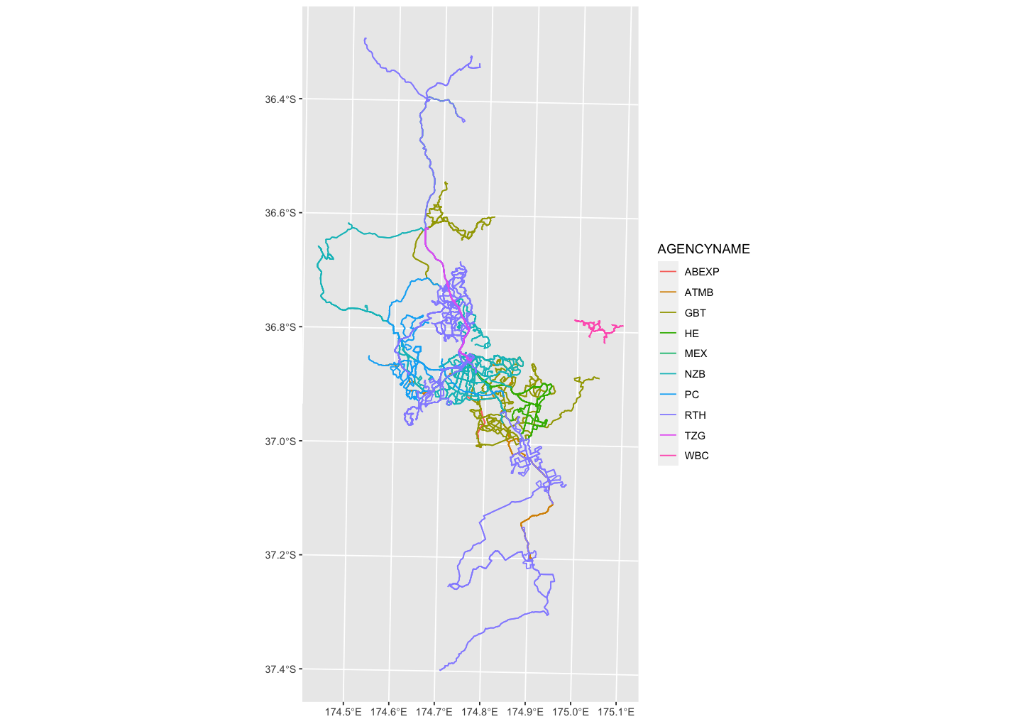
library(sf)akl_bus <- st_read("data/BusService/BusService.shp")#> Reading layer `BusService' from data source `/Users/wany568/Teaching/stats220/lectures/data/BusService/BusService.shp' using driver `ESRI Shapefile'#> Simple feature collection with 509 features and 7 fields#> geometry type: MULTILINESTRING#> dimension: XY#> bbox: xmin: 1727652 ymin: 5859539 xmax: 1787138 ymax: 5982575#> projected CRS: NZGD2000_New_Zealand_Transverse_Mercator_2000data source: Auckland Transport Open GIS Data
- sf: simple features
- spatial data: points, lines from a to b (bus routes), polygons

Reading spatial data*
library(sf)akl_bus <- st_read("data/BusService/BusService.shp")#> Reading layer `BusService' from data source `/Users/wany568/Teaching/stats220/lectures/data/BusService/BusService.shp' using driver `ESRI Shapefile'#> Simple feature collection with 509 features and 7 fields#> geometry type: MULTILINESTRING#> dimension: XY#> bbox: xmin: 1727652 ymin: 5859539 xmax: 1787138 ymax: 5982575#> projected CRS: NZGD2000_New_Zealand_Transverse_Mercator_2000data source: Auckland Transport Open GIS Data

Reading spatial data*
akl_bus[1:4, ]#> Simple feature collection with 4 features and 7 fields#> geometry type: MULTILINESTRING#> dimension: XY#> bbox: xmin: 1751253 ymin: 5915245 xmax: 1758019 ymax: 5921383#> projected CRS: NZGD2000_New_Zealand_Transverse_Mercator_2000#> OBJECTID ROUTEPATTE AGENCYNAME ROUTENAME#> 1 343077 02005 NZB St Lukes To Wynyard Quarter Via Kingsland#> 2 343078 02006 NZB Wynyard Quarter To St Lukes Via Kingsland#> 3 343079 02209 NZB Avondale To City Centre Via New North Rd#> 4 343080 02208 NZB City Centre To Avondale Via New North Rd#> ROUTENUMBE MODE Shape__Len geometry#> 1 20 Bus 7948.418 MULTILINESTRING ((1755487 5...#> 2 20 Bus 7919.198 MULTILINESTRING ((1756321 5...#> 3 22A Bus 11419.588 MULTILINESTRING ((1757613 5...#> 4 22A Bus 11607.711 MULTILINESTRING ((1757346 5...- rich data fmts: audio, images, etc
- seen an unseen file type: google that type and the corresponding r function
Data export ⬆️
From read_*() to write_*()
write_csv(movies_tbl, file = "data/movies.csv")write_sas(movies_tbl, path = "data/movies.sas7bdat")write_json(movies_tbl, path = "data/movies.json")