Atomic vector (1d)
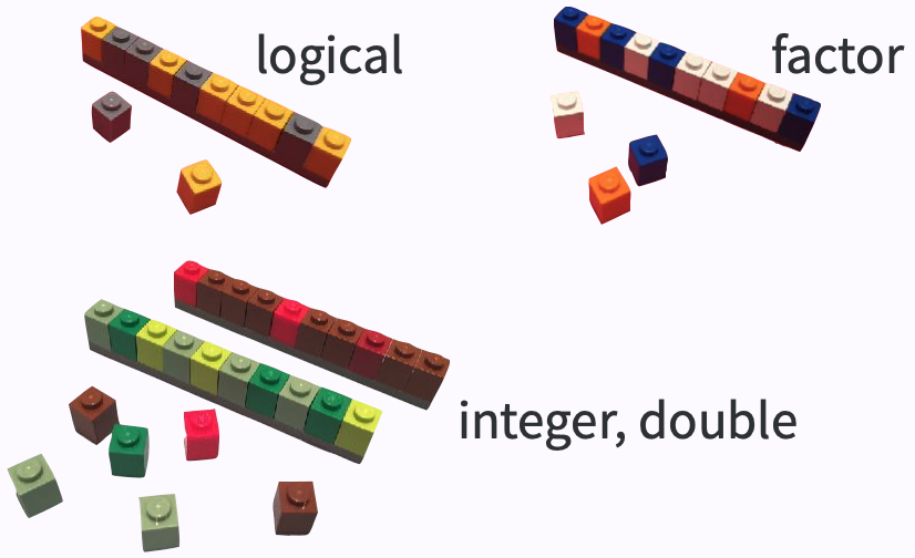
dept <- c("Physics", "Mathematics", "Statistics", "Computer Science")nstaff <- c(12L, 8L, 20L, 23L)image credit: Jenny Bryan
1d ➡️ 2d
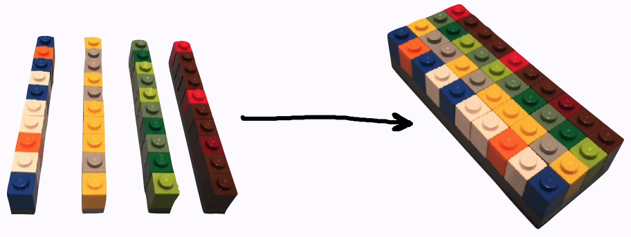
library(tibble)sci_tbl <- tibble( department = dept, count = nstaff, percentage = count / sum(count))sci_tbl#> # A tibble: 4 x 3#> department count percentage#> <chr> <int> <dbl>#> 1 Physics 12 0.190#> 2 Mathematics 8 0.127#> 3 Statistics 20 0.317#> 4 Computer Science 23 0.365image credit: Jenny Bryan
data strs
- lists
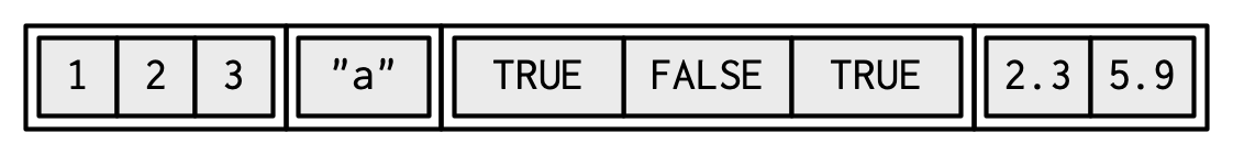
data type
typeof(lst) # primitive type#> [1] "list"data class
class(lst) # type + attributes#> [1] "list"data structure
str(lst)# el can be of diff lengths#> List of 4#> $ : int [1:3] 1 2 3#> $ : chr "a"#> $ : logi [1:3] TRUE FALSE TRUE#> $ : num [1:2] 2.3 5.9data strs
- lists
lst#> [[1]]#> [1] 1 2 3#> #> [[2]]#> [1] "a"#> #> [[3]]#> [1] TRUE FALSE TRUE#> #> [[4]]#> [1] 2.3 5.9
data strs
- lists
Subset by []
lst[1]#> [[1]]#> [1] 1 2 3Subset by [[]]
lst[[1]]#> [1] 1 2 3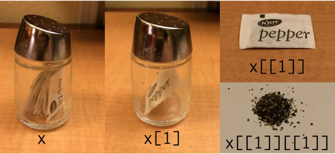
image credit: Hadley Wickham
data strs
- lists
- matrices
- tibbles
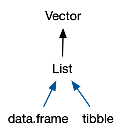
typeof(sci_tbl) # list in essence#> [1] "list"class(sci_tbl) # tibble is a special class of data.frame#> [1] "tbl_df" "tbl" "data.frame"
Reading plain-text rectangular files
(a.k.a. flat or spreadsheet-like files)
- delimited text files with
read_delim().csv: comma separated values withread_csv().tsv: tab separated valuesread_tsv()
.fwf: fixed width files withread_fwf()
head -4 data/pisa/pisa-student.csv # shell command, not R#> year,country,school_id,student_id,mother_educ,father_educ,gender,computer,internet,math,read,science,stu_wgt,desk,room,dishwasher,television,computer_n,car,book,wealth,escs#> 2000,ALB,1001,1,NA,NA,female,NA,no,324.35,397.87,345.66,2.16,yes,no,no,1,3+,1,11-50,-0.6,0.10575582991490981#> 2000,ALB,1001,3,NA,NA,female,NA,no,NA,368.41,385.83,2.16,yes,yes,no,2,0,0,1-10,-1.84,-1.424044581128788#> 2000,ALB,1001,6,NA,NA,male,NA,no,NA,294.17,327.94,2.16,yes,yes,no,2,0,0,1-10,-1.46,-1.306683855365612
Reading comma delimited files
library(readr) # library(tidyverse)pisa <- read_csv("data/pisa/pisa-student.csv", n_max = 2929621)pisa#> # A tibble: 2,929,621 x 22#> year country school_id student_id mother_educ father_educ#> <dbl> <chr> <dbl> <dbl> <lgl> <lgl> #> 1 2000 ALB 1001 1 NA NA #> 2 2000 ALB 1001 3 NA NA #> 3 2000 ALB 1001 6 NA NA #> 4 2000 ALB 1001 8 NA NA #> 5 2000 ALB 1001 11 NA NA #> 6 2000 ALB 1001 12 NA NA #> # … with 2,929,615 more rows, and 16 more variables:#> # gender <chr>, computer <lgl>, internet <chr>,#> # math <dbl>, read <dbl>, science <dbl>, stu_wgt <dbl>,#> # desk <chr>, room <chr>, dishwasher <chr>,#> # television <chr>, computer_n <chr>, car <chr>,#> # book <chr>, wealth <dbl>, escs <dbl>
read_csv() arguments with ?read_csv()
read_csv( file, col_names = TRUE, col_types = NULL, locale = default_locale(), na = c("", "NA"), quoted_na = TRUE, quote = "\"", comment = "", trim_ws = TRUE, skip = 0, n_max = Inf, guess_max = min(1000, n_max), progress = show_progress(), skip_empty_rows = TRUE)![]()
Faster delimited reader at 1.4GB/sec

library(vroom)pisa <- vroom("data/pisa/pisa-student.csv", n_max = 2929621)
Reading proprietary binary files
- Microsoft Excel
.xls: MSFT Excel 2003 and earlier.xlsx: MSFT Excel 2007 and later
library(readxl)time_use <- read_xlsx("data/time-use-oecd.xlsx")time_use#> # A tibble: 461 x 3#> Country Category `Time (minutes)`#> <chr> <chr> <dbl>#> 1 Australia Paid work 211.#> 2 Austria Paid work 280.#> 3 Belgium Paid work 194.#> 4 Canada Paid work 269.#> 5 Denmark Paid work 200.#> 6 Estonia Paid work 231.#> # … with 455 more rows
Reading proprietary binary files
- SAS
.sas7bdatwithread_sas()
- Stata
.dtawithread_dta()
- SPSS
.savwithread_sav()
library(haven)pisa2018 <- read_spss("data/pisa/CY07_MSU_STU_QQQ.sav")Raw PISA data is made available in SAS and SPSS data formats.
data source: https://www.oecd.org/pisa/data/2018database/
Reading chunks for larger than memory data*
chunked <- function(x, pos) { dplyr::filter(x, year == 2018)}pisa2018 <- read_csv_chunked("data/pisa/pisa-student.csv", callback = DataFrameCallback$new(chunked))![]()
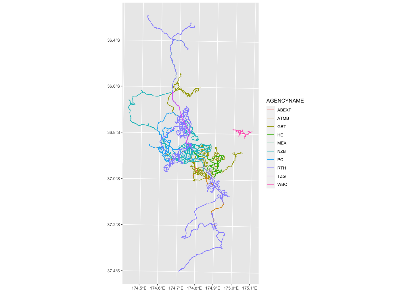
Reading spatial data*
library(sf)akl_bus <- st_read("data/BusService/BusService.shp")#> Reading layer `BusService' from data source `/Users/wany568/Teaching/stats220/lectures/data/BusService/BusService.shp' using driver `ESRI Shapefile'#> Simple feature collection with 509 features and 7 fields#> geometry type: MULTILINESTRING#> dimension: XY#> bbox: xmin: 1727652 ymin: 5859539 xmax: 1787138 ymax: 5982575#> projected CRS: NZGD2000_New_Zealand_Transverse_Mercator_2000data source: Auckland Transport Open GIS Data
![]()
Reading spatial data*
akl_bus[1:4, ]#> Simple feature collection with 4 features and 7 fields#> geometry type: MULTILINESTRING#> dimension: XY#> bbox: xmin: 1751253 ymin: 5915245 xmax: 1758019 ymax: 5921383#> projected CRS: NZGD2000_New_Zealand_Transverse_Mercator_2000#> OBJECTID ROUTEPATTE AGENCYNAME ROUTENAME#> 1 343077 02005 NZB St Lukes To Wynyard Quarter Via Kingsland#> 2 343078 02006 NZB Wynyard Quarter To St Lukes Via Kingsland#> 3 343079 02209 NZB Avondale To City Centre Via New North Rd#> 4 343080 02208 NZB City Centre To Avondale Via New North Rd#> ROUTENUMBE MODE Shape__Len geometry#> 1 20 Bus 7948.418 MULTILINESTRING ((1755487 5...#> 2 20 Bus 7919.198 MULTILINESTRING ((1756321 5...#> 3 22A Bus 11419.588 MULTILINESTRING ((1757613 5...#> 4 22A Bus 11607.711 MULTILINESTRING ((1757346 5...