Assignment 1
This assignment is due 23:59 Friday 26 March (NZDT).
- You should submit an R file (i.e. file extension
.R) containing R code that assigns the appropriate values to the appropriate symbols. - Your R file will be executed in order and checked against the values that have been assigned to the relevant symbols using an automatic grading system. Marks will be fully deducted for non-identical results.
- Intermediate steps to achieve the final results will NOT be checked.
- Each question is worth 1 point.
- You should submit your R file on Canvas.
- Late assignments are NOT accepted unless prior arrangement for medical/compassionate reasons.
In this assignment, your are going to work with 2018 Citi Bike trip data
in New York City (2018-citibike-tripdata.csv). The data includes:
- Trip Duration (seconds)
- Start Time and Date
- Stop Time and Date
- Start Station Name
- End Station Name
- Station ID
- Station Lat/Long
- Bike ID
- User Type (Customer = 24-hour pass or 3-day pass user; Subscriber = Annual Member)
- Gender (Zero=unknown; 1=male; 2=female)
- Year of Birth
You shall use the following packages for this assignment:
library(tidyverse)
- Make sure to include the snippet above upfront in your R file.
- DO NOT include
install.packages()in your R file.
Suppose that you have created an Rproj for this course. You need to
download 2018-citibike-tripdata.csv
here
to data/ under your Rproj.
- You’re required to use relative file paths
data/2018-citibike-tripdata.csvto import the data. - NO marks will be given for using URL links or different file paths.
- DO NOT apply any
theme()and aesthetics other than what I asked to your plots. - DO NOT print any R objects and plots.
Question 1
Read data/2018-citibike-tripdata.csv into R. You should end up with a
tibble called nycbikes18_raw.
nycbikes18_raw
#> # A tibble: 333,687 x 15
#>    tripduration starttime           stoptime
#>           <dbl> <dttm>              <dttm>
#>  1          932 2018-01-01 07:06:17 2018-01-01 07:21:50
#>  2          550 2018-01-01 17:06:18 2018-01-01 17:15:28
#>  3          510 2018-01-01 17:06:56 2018-01-01 17:15:27
#>  4          354 2018-01-01 19:53:10 2018-01-01 19:59:05
#>  5          250 2018-01-01 22:34:30 2018-01-01 22:38:40
#>  6          613 2018-01-02 03:05:05 2018-01-02 03:15:19
#>  7          290 2018-01-02 17:13:51 2018-01-02 17:18:42
#>  8          381 2018-01-02 17:50:03 2018-01-02 17:56:24
#>  9          318 2018-01-02 18:55:58 2018-01-02 19:01:16
#> 10         1852 2018-01-02 21:55:29 2018-01-02 22:26:22
#> # … with 333,677 more rows, and 12 more variables:
#> #   start_station_id <dbl>, start_station_name <chr>,
#> #   start_station_latitude <dbl>, start_station_longitude <dbl>,
#> #   end_station_id <dbl>, end_station_name <chr>,
#> #   end_station_latitude <dbl>, end_station_longitude <dbl>,
#> #   bikeid <dbl>, usertype <chr>, birth_year <dbl>, gender <dbl>
Question 2
Regarding nycbikes18_raw, you are interested in the total number of
bike trips ridden by each age group and user type. Plot a bar chart to
address the question of interest. You should end up with a ggplot
object called p1, with
colour = "white".
p1
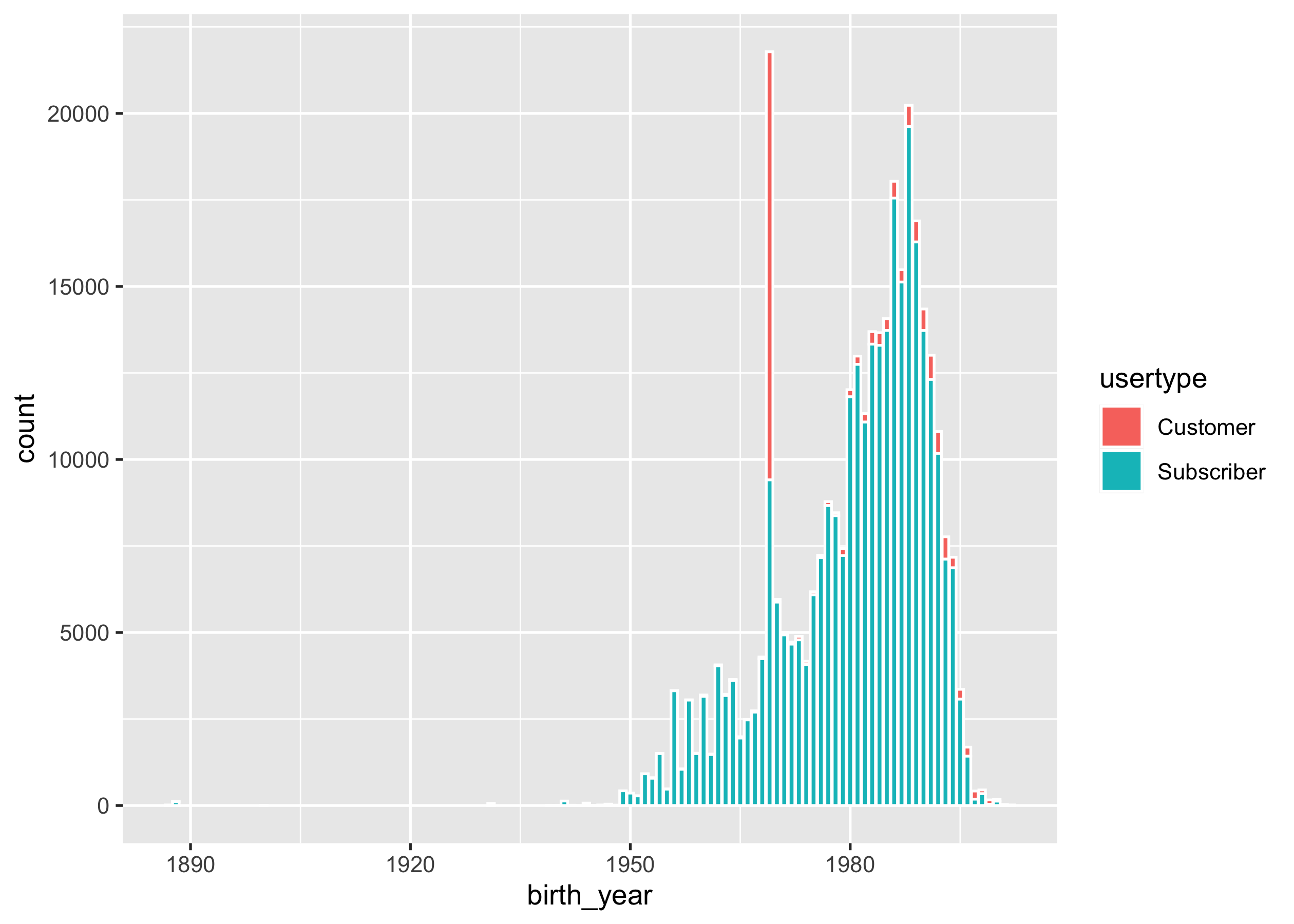
Question 3
From the above plot p1, it is noted that there are a few trips done by
users who were born before 1900. These users possibly don’t want to
reveal their ages. You need to remove these observations with
birth_year greater than 1900 for the rest of the analysis. You
should end up with a tibble called nycbikes18.
nycbikes18
#> # A tibble: 333,557 x 15
#>    tripduration starttime           stoptime
#>           <dbl> <dttm>              <dttm>
#>  1          932 2018-01-01 07:06:17 2018-01-01 07:21:50
#>  2          550 2018-01-01 17:06:18 2018-01-01 17:15:28
#>  3          510 2018-01-01 17:06:56 2018-01-01 17:15:27
#>  4          354 2018-01-01 19:53:10 2018-01-01 19:59:05
#>  5          250 2018-01-01 22:34:30 2018-01-01 22:38:40
#>  6          613 2018-01-02 03:05:05 2018-01-02 03:15:19
#>  7          290 2018-01-02 17:13:51 2018-01-02 17:18:42
#>  8          381 2018-01-02 17:50:03 2018-01-02 17:56:24
#>  9          318 2018-01-02 18:55:58 2018-01-02 19:01:16
#> 10         1852 2018-01-02 21:55:29 2018-01-02 22:26:22
#> # … with 333,547 more rows, and 12 more variables:
#> #   start_station_id <dbl>, start_station_name <chr>,
#> #   start_station_latitude <dbl>, start_station_longitude <dbl>,
#> #   end_station_id <dbl>, end_station_name <chr>,
#> #   end_station_latitude <dbl>, end_station_longitude <dbl>,
#> #   bikeid <dbl>, usertype <chr>, birth_year <dbl>, gender <dbl>
‼️ You shall work with nycbikes18 for the rest of the assignment.
Question 4
Calculate the total trip durations over the year. You should end up with
a double called ttl_tripd.
ttl_tripd
#> [1] 226912929
Question 5
Find out the number of Citi bikes used in 2018. You should end up with
an integer called n_bikes. (HINTS: You may find unique()
useful.)
n_bikes
#> [1] 900
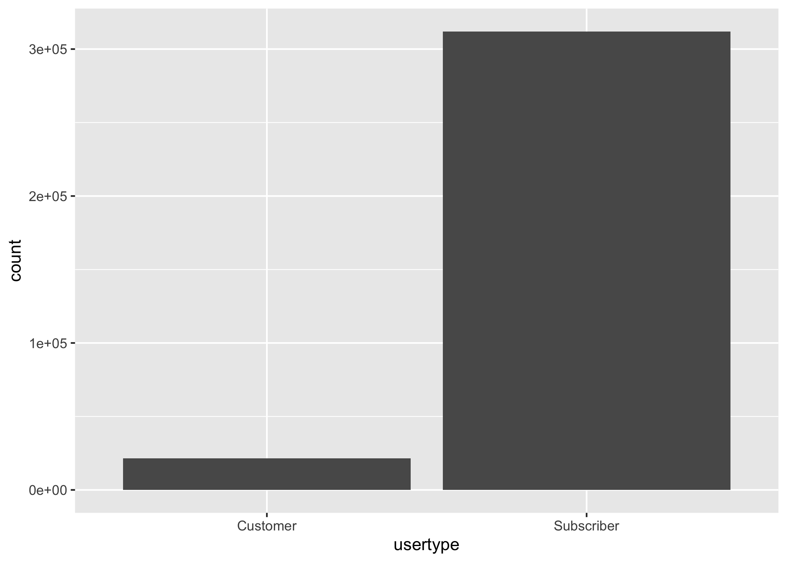
Question 6
You’d like to know if Citi bike subscribers ride more often than
one-time customers. Present a bar chart for the tallies of trips by each
usertype. You should end up with a ggplot object called p2.
p2
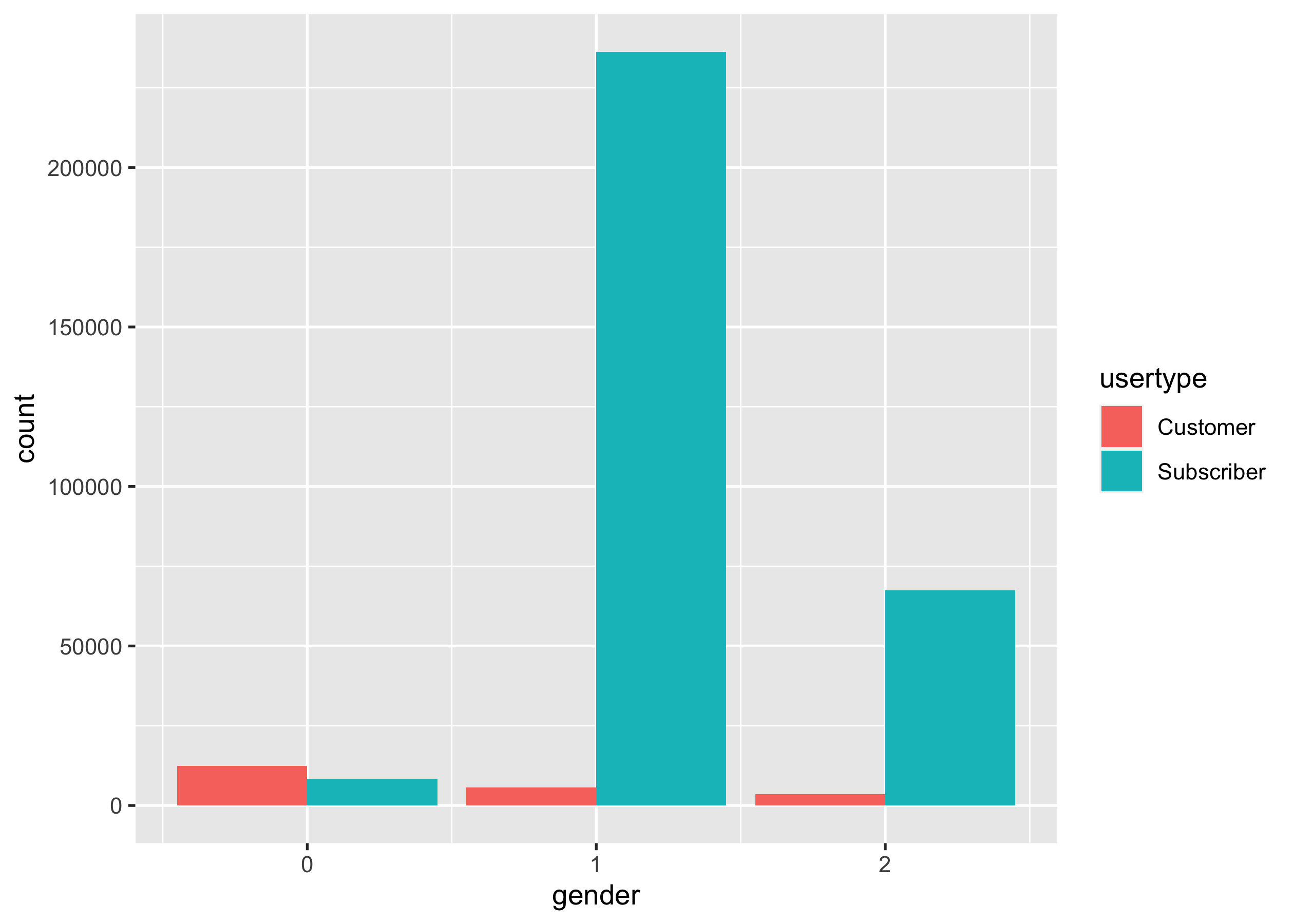
Question 7
You’re interested in riding behaviours of users of different genders
based on their user types. Produce a side-by-side bar charts to display
the tallies of trips by each gender, grouped by usertype. You should
end up with a ggplot object called p3.
p3
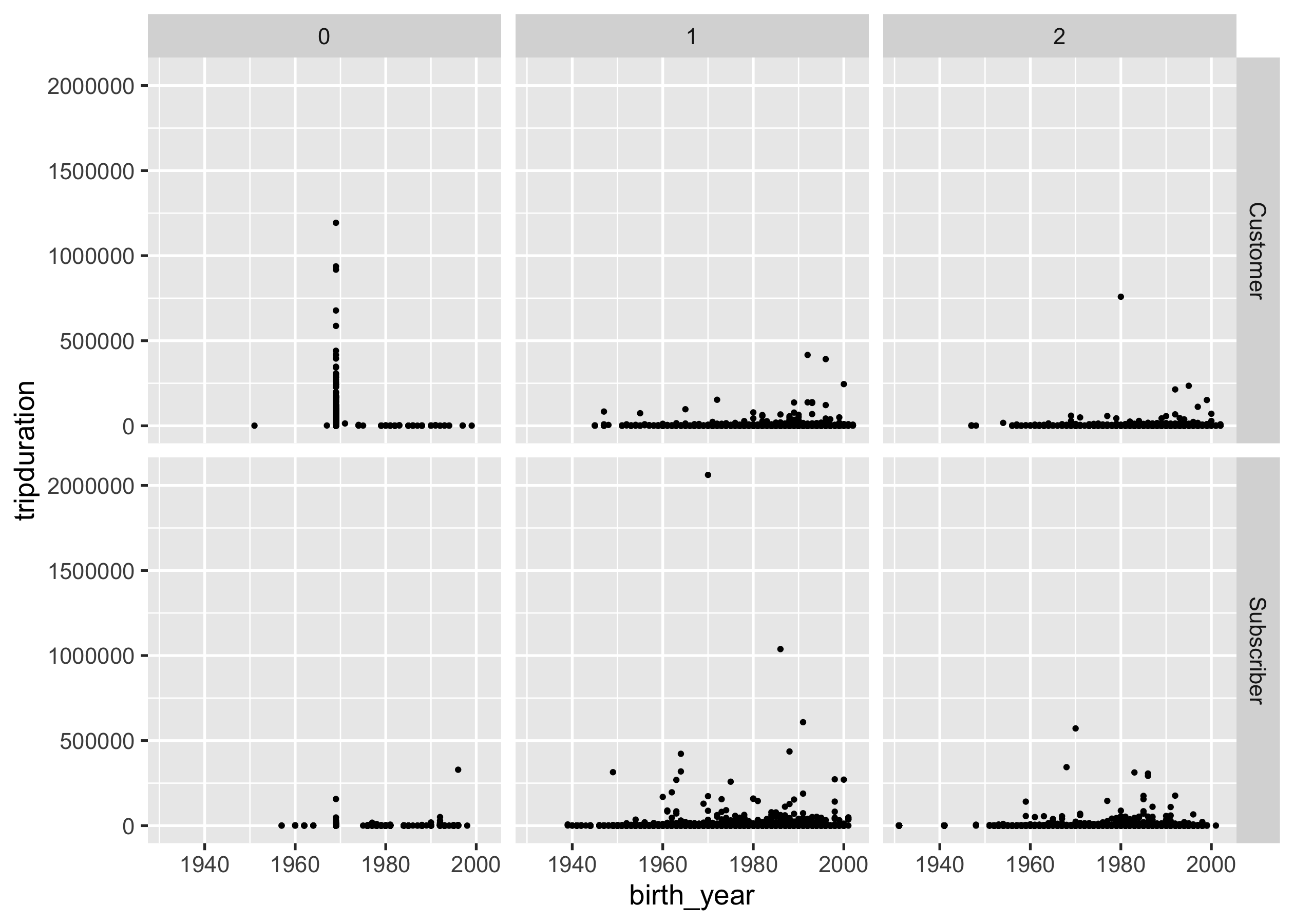
Question 8
Do younger users ride for longer trips? Generate a scatter plot with
birth_year on x axis and tripduration on y axis, faceted by
usertype on rows and gender on columns. You should end up with a
ggplot object named p4 with
size = 0.5.
p4
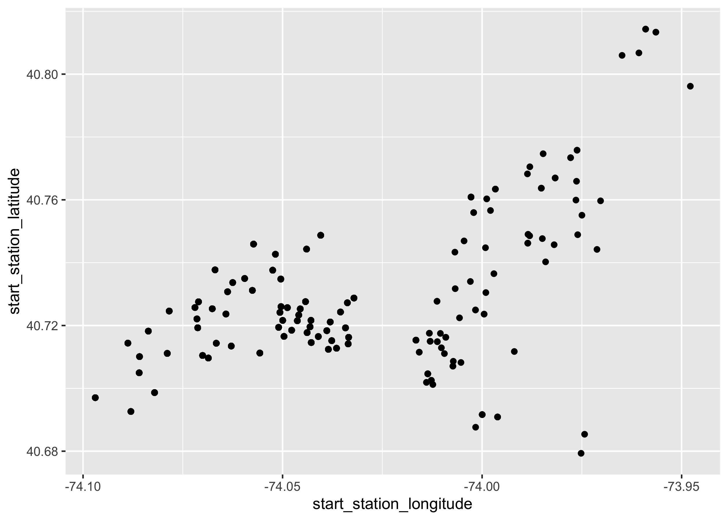
Question 9
Let’s take a look at where Citi bike stations are located. Plot the
following layered graphics: (1) overlaying points indicate all
geographical locations of start stations; (2) one more layer of points
represent all end stations, on top of the first layer. You should end up
with a ggplot object named p5.
p5
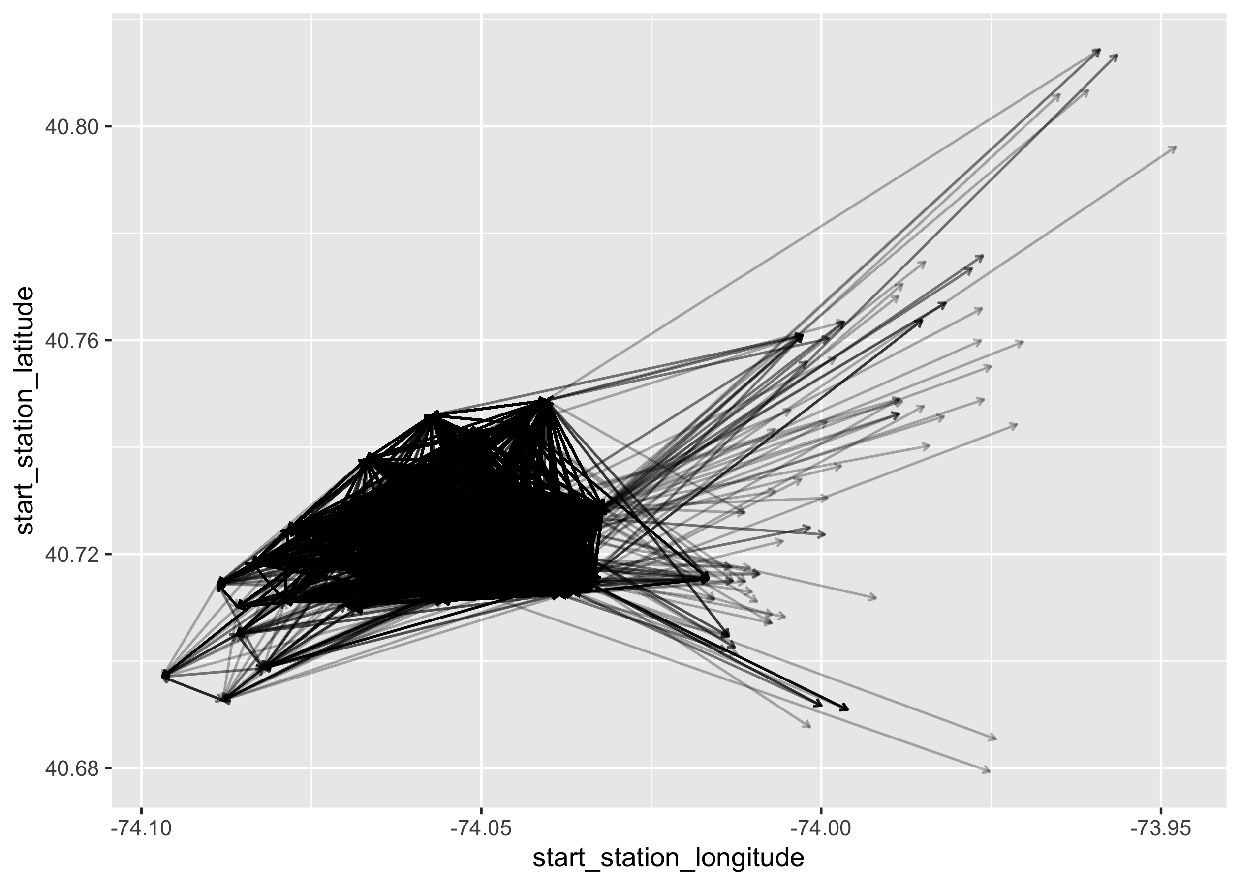
Question 10
To get a picture of how Citi bikes flow from one place to another, you
need to plot all bike trips with arrows pointing from start to end
stations. You should end up with a ggplot object named p6, with
arrow = arrow(length = unit(0.01, "npc")),alpha = 0.3.
HINTS: check out the
?geom_segment
for examples.
p6