Lab 04 Solution
This lab exercise is due 23:59 Wednesday 7 April (NZST).
- You should submit an R file (i.e. file extension
.R) containing R code that assigns the appropriate values to the appropriate symbols. - Your R file will be executed in order and checked against the values that have been assigned to the symbols using an automatic grading system. Marks will be fully deducted for non-identical results.
- Intermediate steps to achieve the final results will NOT be checked.
- Each question is worth 0.2 points.
- You should submit your R file on Canvas.
- Late assignments are NOT accepted unless prior arrangement for medical/compassionate reasons.
In this lab exercise, you are going to work with two data sets:
step-count.csv that contains Dr Wang’s hourly step counts, and
location.csv with cities where she was in 2019. You shall use the
following code snippet (and include them upfront in your R file) to
start with this lab session:
library(tidyverse)
step_count_raw <- read_csv("data/step-count/step-count.csv",
  locale = locale(tz = "Australia/Melbourne"))
location <- read_csv("data/step-count/location.csv")
step_count_raw
#> # A tibble: 5,448 x 3
#>    `Date/Time`         Date       `Step Count (count)`
#>    <dttm>              <date>                    <dbl>
#>  1 2019-01-01 09:00:00 2019-01-01                  764
#>  2 2019-01-01 10:00:00 2019-01-01                  913
#>  3 2019-01-02 00:00:00 2019-01-02                    9
#>  4 2019-01-02 10:00:00 2019-01-02                 2910
#>  5 2019-01-02 11:00:00 2019-01-02                 1390
#>  6 2019-01-02 12:00:00 2019-01-02                 1020
#>  7 2019-01-02 13:00:00 2019-01-02                  472
#>  8 2019-01-02 15:00:00 2019-01-02                 1220
#>  9 2019-01-02 16:00:00 2019-01-02                 1670
#> 10 2019-01-02 17:00:00 2019-01-02                 1390
#> # … with 5,438 more rows
location
#> # A tibble: 21 x 2
#>    date       location
#>    <date>     <chr>
#>  1 2019-01-15 Austin
#>  2 2019-01-16 Austin
#>  3 2019-01-17 Austin
#>  4 2019-01-18 Austin
#>  5 2019-01-19 Austin
#>  6 2019-01-20 Austin
#>  7 2019-01-21 Austin
#>  8 2019-01-22 Austin
#>  9 2019-01-23 Austin
#> 10 2019-01-24 Austin
#> # … with 11 more rows
Suppose that you have created an Rproj for this course. You need to
download step-count.csv
here
and location.csv
here,
to data/step-count/ under your Rproj folder.
- You’re required to use relative file paths
data/step-count/step-count.csvanddata/step-count/location.csvto import these data. - NO marks will be given for using URL links or different file paths.
- DO NOT include
install.packages()in your R file. - DO NOT print any R objects and plots.
Question 1
Change the column names of step_count_raw to date_time, date, and
count. You should end up with a tibble called step_count.
step_count <- step_count_raw %>%
  rename(
    date_time = `Date/Time`,
    date = Date,
    count = `Step Count (count)`
  )
step_count
#> # A tibble: 5,448 x 3
#>    date_time           date       count
#>    <dttm>              <date>     <dbl>
#>  1 2019-01-01 09:00:00 2019-01-01   764
#>  2 2019-01-01 10:00:00 2019-01-01   913
#>  3 2019-01-02 00:00:00 2019-01-02     9
#>  4 2019-01-02 10:00:00 2019-01-02  2910
#>  5 2019-01-02 11:00:00 2019-01-02  1390
#>  6 2019-01-02 12:00:00 2019-01-02  1020
#>  7 2019-01-02 13:00:00 2019-01-02   472
#>  8 2019-01-02 15:00:00 2019-01-02  1220
#>  9 2019-01-02 16:00:00 2019-01-02  1670
#> 10 2019-01-02 17:00:00 2019-01-02  1390
#> # … with 5,438 more rows
Question 2
Join the second data location to the primary data step_count. You
should end up with a tibble called step_count_loc.
step_count_loc <- step_count %>%
  left_join(location)
step_count_loc
#> # A tibble: 5,448 x 4
#>    date_time           date       count location
#>    <dttm>              <date>     <dbl> <chr>
#>  1 2019-01-01 09:00:00 2019-01-01   764 <NA>
#>  2 2019-01-01 10:00:00 2019-01-01   913 <NA>
#>  3 2019-01-02 00:00:00 2019-01-02     9 <NA>
#>  4 2019-01-02 10:00:00 2019-01-02  2910 <NA>
#>  5 2019-01-02 11:00:00 2019-01-02  1390 <NA>
#>  6 2019-01-02 12:00:00 2019-01-02  1020 <NA>
#>  7 2019-01-02 13:00:00 2019-01-02   472 <NA>
#>  8 2019-01-02 15:00:00 2019-01-02  1220 <NA>
#>  9 2019-01-02 16:00:00 2019-01-02  1670 <NA>
#> 10 2019-01-02 17:00:00 2019-01-02  1390 <NA>
#> # … with 5,438 more rows
sum(is.na(step_count_loc$location))
#> [1] 5125
Question 3
Replace missing values with "Melbourne" in the location column of
the step_count_loc. You should end up with a tibble called
step_count_full.
# NO mark given to Q2, if you do the following line:
# step_count_loc$location[is.na(step_count_loc$location)] <- "Melbourne"
step_count_full <- step_count_loc %>%
  mutate(location = case_when(
    is.na(location) ~ "Melbourne",
    TRUE ~ location))
step_count_full
#> # A tibble: 5,448 x 4
#>    date_time           date       count location
#>    <dttm>              <date>     <dbl> <chr>
#>  1 2019-01-01 09:00:00 2019-01-01   764 Melbourne
#>  2 2019-01-01 10:00:00 2019-01-01   913 Melbourne
#>  3 2019-01-02 00:00:00 2019-01-02     9 Melbourne
#>  4 2019-01-02 10:00:00 2019-01-02  2910 Melbourne
#>  5 2019-01-02 11:00:00 2019-01-02  1390 Melbourne
#>  6 2019-01-02 12:00:00 2019-01-02  1020 Melbourne
#>  7 2019-01-02 13:00:00 2019-01-02   472 Melbourne
#>  8 2019-01-02 15:00:00 2019-01-02  1220 Melbourne
#>  9 2019-01-02 16:00:00 2019-01-02  1670 Melbourne
#> 10 2019-01-02 17:00:00 2019-01-02  1390 Melbourne
#> # … with 5,438 more rows
step_count_full %>%
  slice(90:95)
#> # A tibble: 6 x 4
#>   date_time           date        count location
#>   <dttm>              <date>      <dbl> <chr>
#> 1 2019-01-14 17:00:00 2019-01-14   65.7 Melbourne
#> 2 2019-01-14 19:00:00 2019-01-14   22   Melbourne
#> 3 2019-01-14 20:00:00 2019-01-14    1   Melbourne
#> 4 2019-01-15 03:00:00 2019-01-15    8   Austin
#> 5 2019-01-15 05:00:00 2019-01-15  355   Austin
#> 6 2019-01-15 06:00:00 2019-01-15 1800   Austin
Question 4
Aggregate the hourly data step_count_full to daily step counts. You
should end up with a tibble called step_count_daily.
step_count_daily <- step_count_full %>%
  group_by(date) %>%
  summarise(daily_count = sum(count))
step_count_daily
#> # A tibble: 364 x 2
#>    date       daily_count
#>    <date>           <dbl>
#>  1 2019-01-01       1677
#>  2 2019-01-02      14987
#>  3 2019-01-03       9424
#>  4 2019-01-04          9
#>  5 2019-01-05       7359
#>  6 2019-01-06         21
#>  7 2019-01-07       9057.
#>  8 2019-01-08      10341
#>  9 2019-01-09       6394
#> 10 2019-01-10       7489
#> # … with 354 more rows
Question 5
Subset step_count_daily with daily counts that are greater than or
equal to 10,000 steps. You should end up with a tibble called
step_count_10000.
step_count_10000 <- step_count_daily %>%
  filter(daily_count >= 10000)
step_count_10000
#> # A tibble: 108 x 2
#>    date       daily_count
#>    <date>           <dbl>
#>  1 2019-01-02      14987
#>  2 2019-01-08      10341
#>  3 2019-01-22      15579
#>  4 2019-01-23      15362
#>  5 2019-01-31      11287.
#>  6 2019-02-15      10117
#>  7 2019-02-21      10312
#>  8 2019-02-26      12005
#>  9 2019-03-01      14510
#> 10 2019-03-05      11754.
#> # … with 98 more rows
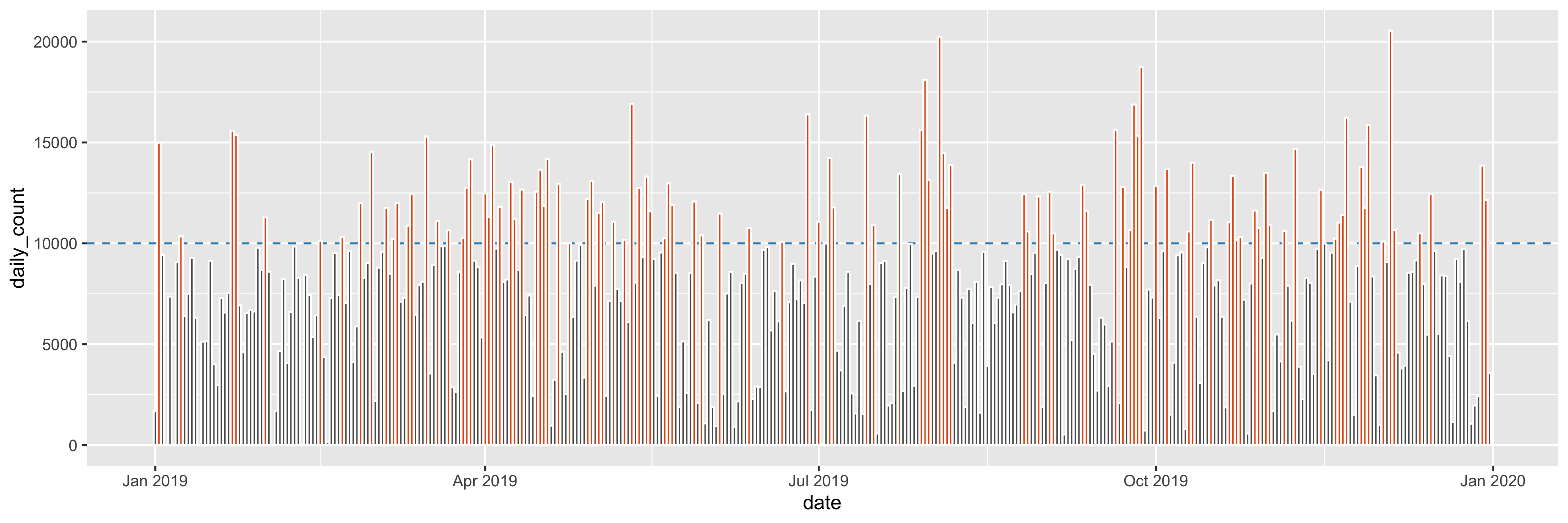
Question4fun (NO marks)
Plot daily counts over the year of 2019 and highlight these daily counts that are greater than or equal to 10,000.
- horizon line:
colour = "#2b8cbe", andlinetype = "dashed" - bar:
fill = "#e6550d", andcolour = "white"
step_count_daily %>%
  ggplot(aes(date, daily_count)) +
  geom_hline(yintercept = 10000, colour = "#2b8cbe", linetype = "dashed") +
  geom_col(colour = "white") +
  geom_col(data = step_count_10000, fill = "#e6550d", colour = "white")